
Inside the PyTorch Compiler
There are two types of deep learning frameworks - eager mode and graph mode. PyTorch is an example of eager mode framework while TensorFlow (at least till 1.x versions) is an example of graph mode framework.
In graph model frameworks, we define a static computation graph of tensors and operations on those tensors. The framework then executes this graph during training/inference. Since the graph is static (does not change at runtime), the framework can optimize the graph before execution. We shall discuss the types of optimizations later.
In contrast, in eager mode, a graph of tensors and operations is created/expanded dynamically as each operation is executed on the tensors. Which means, every forward pass creates a new execution graph from scratch.
The advantage of eager mode is that programmers are not restricted to a rigid API and can leverage all features of Python while describing their computation. For example, they can use arbitrary conditionals (if statements) as part of their model. The appropriate graph will be constructed at runtime based on the chosen conditional branch. Another example is the ability to use print statements or debuggers.
One big downside of the eager mode is that the framework cannot optimize the execution graph for you (since it can change on every forward pass). This downside has recently become a significant issue as models have grown in their number of parameters and computations. In the current era of billion parameter models, compute efficiency is as important (if not more) as developer productivity. Plain eager mode (at the cost of development efficiency) can add a large overhead due to sub-optimal programmer code, just in time Python compilation, inefficient use of GPU layout, frequent and unnecessary memory reads and writes between individual GPU kernel executions, etc.
To address these new requirements, PyTorch 2 introduces two new extensions - TorchDynamo and TorchInductor. With these, it attempts to leverage the best of both worlds - the productivity of eager mode combined with the efficiency of pre-compiled execution graphs.
Graph Breaks
The core idea behind these extensions is to break the execution graph into multiple subgraphs where is subgraph is guaranteed to be static at runtime. Then each subgraph can be compiled, cached and reused.
For example, consider the following simplified computation on a scalar tensor.
def leaky_relu(a):
    if a > 0:
        return a
    return 0.1 * a

if __name__ == "__main__":
    data = torch.randn((1,))
    leaky_relu(data)
The graph of operations in this model includes a data dependent conditional statement and therefore cannot be pre-compiled. Graph mode frameworks do not allow such operations.
TorchDynamo in PyTorch 2 resolves this issue by breaking the computation into three sub graph. The first graph corresponds to operations before the conditional statement and the other two graphs correspond to the two branches. Each subgraph can be independently optimised and cached. The following block shows the three FX subgraphs (FX is a representation of a graph of operations on Tensors in PyTorch. It has enough information to reconstruct the computation source code based on the graph and therefore useful as an intermediate representation for compilers).
FX Graph 1:
opcode         name    target                  args       kwargs
-------------  ------  ----------------------  ---------  --------
placeholder    l_a_    L_a_                    ()         {}
call_function  gt      <built-in function gt>  (l_a_, 0)  {}
output         output  output                  ((gt,),)   {}

FX Graph 2: (if output == True)
Skipped because of no content

FX Graph 3: (if output == False)
opcode         name    target                   args         kwargs
-------------  ------  -----------------------  -----------  --------
placeholder    l_a_    L_a_                     ()           {}
call_function  mul     <built-in function mul>  (0.1, l_a_)  {}
output         output  output                   ((mul,),)    {}
TorchDynamo
Essentially, TorchDynamo is a Just-In-Time (JIT) compiler that analyses Python bytecode line by line to construct an FX graph till it reaches a point which could be a reason for graph break. For example, the block below shows the Python bytecode for the simple model described before.
0 LOAD_FAST                0 (a)
2 LOAD_CONST               1 (0)
4 COMPARE_OP               4 (>)
6 POP_JUMP_IF_FALSE        6 (to 12)

8 LOAD_FAST                0 (a)
10 RETURN_VALUE

12 LOAD_CONST              2 (0.1)
14 LOAD_FAST               0 (a)
16 BINARY_MULTIPLY
18 RETURN_VALUE
Dynamo iterates through this bytecode one by one till it reaches the bytecode POP_JUMP_IF_FALSE at byte position 6. POP_JUMP_IF_FALSE decides which code path will be chosen next based on output of bytecode COMPARE_OP. The chosen path could either be byte positions 8 to 10, or, byte position 12 to 18.
Since the output of COMPARE_OP is not known in advance (it depends on data at runtime), Dynamo stops at this point to create the first subgraph. The traced graph till now looks like the following code.
FX Graph 1:
opcode         name    target                  args       kwargs
-------------  ------  ----------------------  ---------  --------
placeholder    l_a_    L_a_                    ()         {}
call_function  gt      <built-in function gt>  (l_a_, 0)  {}
output         output  output                  ((gt,),)   {}

===== Generated code based on FX Graph 1 (__compiled_fn_0) =====
class GraphModule(torch.nn.Module):
    def forward(self, L_a_ : torch.Tensor):
        l_a_ = L_a_
        gt = l_a_ > 0;  l_a_ = None
        return (gt,)
This graph does not have any data dependent operations or conditional branches. Therefore, a separate compiler (like Torch Inductor) can aggressively optimize this subgraph and the optimized compiled code can be cached and reused at runtime.
Dynamo then modifies the original bytecode to include a call to __compiled_fn_0 as shown below.
0 LOAD_GLOBAL              0 (__compiled_fn_0)
2 LOAD_FAST                0 (a)
4 CALL_FUNCTION            1
6 UNPACK_SEQUENCE          1
8 POP_JUMP_IF_FALSE        9 (to 18)
10 LOAD_GLOBAL             1 (__resume_at_8_1)
12 LOAD_FAST               0 (a)
14 CALL_FUNCTION           1
16 RETURN_VALUE
18 LOAD_GLOBAL             2 (__resume_at_12_2)
20 LOAD_FAST               0 (a)
22 CALL_FUNCTION           1
24 RETURN_VALUE
Here __resume_at_8_1 and __resume_at_12_2 are called continuation functions and they just load the bytecode sequence from the original bytecode source starting at line 8 and 12 respectively as shown below.
===== __resume_at_8_1 =====
8 LOAD_FAST                0 (a)
10 RETURN_VALUE

===== __resume_at_12_2 =====
12 LOAD_CONST              2 (0.1)
14 LOAD_FAST               0 (a)
16 BINARY_MULTIPLY
18 RETURN_VALUE
Dynamo then continues along each path - __resume_at_8_1 and __resume_at_12_2 to analyze and generate remaining subgraphs. Since __resume_at_8_1 does not have any content, Dynamo skips it. The branch __resume_at_12_2 results in the following subgraph.
FX Graph 3:
opcode         name    target                   args         kwargs
-------------  ------  -----------------------  -----------  --------
placeholder    l_a_    L_a_                     ()           {}
call_function  mul     <built-in function mul>  (0.1, l_a_)  {}
output         output  output                   ((mul,),)    {}

===== Generated code based on FX Graph 3 (__compiled_fn_3) =====
class GraphModule(torch.nn.Module):
    def forward(self, L_a_ : torch.Tensor):
        l_a_ = L_a_
        mul = 0.1 * l_a_;  l_a_ = None
        return (mul,)
The corresponding modified bytecode to include call to __compiled_fn_3 is shown below.
0 LOAD_GLOBAL              0 (__compiled_fn_3)
2 LOAD_FAST                0 (a)
4 CALL_FUNCTION            1
6 UNPACK_SEQUENCE          1
8 RETURN_VALUE
The final bytecode is shown below.
0 LOAD_GLOBAL              0 (__compiled_fn_0)
2 LOAD_FAST                0 (a)
4 CALL_FUNCTION            1
6 UNPACK_SEQUENCE          1
8 POP_JUMP_IF_FALSE        7 (to 14)
10 LOAD_FAST               0 (a)
12 RETURN_VALUE
14 LOAD_GLOBAL             0 (__compiled_fn_3)
16 LOAD_FAST               0 (a)
18 CALL_FUNCTION           1
20 UNPACK_SEQUENCE         1
22 RETURN_VALUE
Here __compiled_fn_0 and __compiled_fn_3 are supposed to be optimized code generated with a compiler based on FX subgraphs.
At this point, the entire process seems slow and generates worse output for the toy example we used. Dynamo also generates certain guards that ensure that the compiled and cached function can be reused on the next input. These generated guard function check a combination of aspects of input tensors like size, shape, requires_grad attribute, the backend compiler used, etc. If the guard function fails on the next input, the compiled code may no longer be valid for that input and the code is recompiled for the new input. This adds additional latency.
But for real world use cases, especially in modules with minimal graph breaks, compilers can generate highly optimized kernels for subgraphs. Once generated, these kernels are cached and reused. For example, TorchInductor (the built in compiler in PTorch 2) uses a concept called operator fusion to generate GPU kernels that minimize memory transfers within the GPU when performing a sequence of operations on data. Such optimizations can dramatically speed up large models by making them compute bound rather than being IO bound.
AOTAutoGrad
In previous section, we saw an example of how dynamo constructs FX graphs of forward pass through a module. But during training, we also want to create and optimize a graph for the backward pass.
Usually, in eager mode, PyTorch uses reverse mode automatic differentiation to record all operations in forward pass and create the backward graph dynamically. But to optimize training, we need a static graph of operations of the backward graph too.
To obtain that, PyTorch 2 includes another extension called AOTAutograd. AOTAutograd uses the code obtained from forward pass FX graph and passes fake tensors through it in eager mode. It then calls the backward method on the output and records all operations (during forward and backward pass) in a joint graph. AOTAutograd then uses the min-cut algorithm to partition the graph into two parts - forward pass and backward pass. These may not be same as the user defined forward and backward passes as the partitioning algorithm decides which operations should go where.
In case of graph breaks, each of the subgraph generates a forward and backward graph independently. For instance, for FX graph 3 in previous example, AOTAutograd generates the following joint, forward and backward graphs.
==== Joint graph 4 =====
def forward(self, primals, tangents):
    primals_1: "f32[1]"; tangents_1: "f32[1]";
    primals_1, tangents_1, = fx_pytree.tree_flatten_spec([primals, tangents], self._in_spec)
    mul: "f32[1]" = torch.ops.aten.mul.Tensor(primals_1, 0.1);  primals_1 = None
    mul_1: "f32[1]" = torch.ops.aten.mul.Tensor(tangents_1, 0.1);  tangents_1 = None
    return pytree.tree_unflatten([mul, mul_1], self._out_spec)

TRACED GRAPH
===== Forward graph 4 =====
def forward(self, primals_1: "f32[1]"):
    mul: "f32[1]" = torch.ops.aten.mul.Tensor(primals_1, 0.1);  primals_1 = None
    return [mul]

TRACED GRAPH
===== Backward graph 4 =====
def forward(self, tangents_1: "f32[1]"):
    mul_1: "f32[1]" = torch.ops.aten.mul.Tensor(tangents_1, 0.1);  tangents_1 = None
    return [mul_1]
All these subgraphs can be optimized and cached by a backend compiler. Note that TorchDynamo just creates static subgraphs and transforms the bytecode to use their reconstructed code. To make the code faster, it needs to be paired with a compiler that can generate optimized code for the static subgraphs. TorchInductor, PyTorch’s built in backend compiler, uses these subgraphs to generate optimized C++ code or Triton kernels depending on the hardware.
Aten Operators
Note that the output code of AOTAutograd looks different and more primitive than one generated by Dynamo. The reason is that both output core using different sets of operations. There are three broad sets of operators in PyTorch -
- Torch operations - This is the set of all operations defined in PyTorch. The Dynamo regenerated code from FX graph uses these operations. The operations in this set are at a much higher abstraction for a compiler to translate and work with efficiently. Moreover, this set has a large number of operations and new operators are added all the time.
- Aten operations - This is a lower level tensor operations library which has a much smaller set of primitive tensor operations. All PyTorch operations can be decomposed into a sequence of aten operations. For instance
torch.nn.Hardsigmoidcan be replaced withaten.hardsigmoid. This set still contains hundreds of operators. - Aten core opset - This is a smaller subset of about 250 aten operations. These operations are also purely functional (no inplace mutations). All aten operations can be decomposed into a sequence of aten core opset. For instance,
aten.hardsigmoidcan be further decomposed intoaten.clamp(aten.clamp(self + 3, min=0), max=6) / 6
AOTAutograd rewrites the forward and backward graphs in aten core opset. It also guarantees data type and shape meta information (for example, f32[1] shows the data type and shape of the tensor). For dynamic shapes, shape information is stored using symbolic variables. Operations like broadcasting, type conversions, etc. are made explicit.
Such intermediate representation (IR), built using a small set of operations and associated data type and shape information, helps the compilers translate the code into optimized target specific output. Such incremental decomposition from higher level user code into lower level intermediate representations is a common part of any compilation process.
Graph Optimizations
The output IR of TorchDynamo/AOTAutograd can be used with a number of supported backend compilers. PyTorch 2 also includes a built in compiler named TorchInductor. Apart from basic compiler optimizations (like constant folding, common subexpression elimination, etc.), these compilers focus on two core areas relevant to deep learning - operator fusion and tiling. Both attempt to minimize IO operations on the device memory essentially ensuring that none of the threads are idle. Compilers also perform other important optimizations like activation checkpointing, intelligent quantization, device specific optimizations like using CUDA graphs for reducing kernel launch overhead, and more.
Operator Fusion
In PyTorch’s eager mode, every operation launches a new kernel on the target device. The lifecycle of every kernel involves three stages - reading data from memory, executing the operation, writing the output back to memory. Often, execution is the fastest part of this cycle. Therefore, to increase the efficiency, we need to minimize the loading and storing of data from memory.
GPUs have a slightly different memory hierarchy than CPUs. In GPUs, each thread has its own local memory which is registers. Multiple threads are grouped into blocks. Each block has an separate memory that is shared between all threads of that block. The shared memory cannot be used to share data between threads of different blocks. GPU also has an L2 cache which is shared between multiple streaming multiprocessors (SM). L2 cache can be used to share data between threads of different blocks. Finally, the GPU also has a global memory that is much larger than L2 cache which is also shared among all blocks. Reading from and writing to shared memory is orders of magnitude faster compared to global memory. Therefore, if a kernel only reads data that was written by the immediately previous kernel, there is no need to write that data back to the global memory. The computations of both kernels can be fused such that intermediate data is stored in the shared or thread local memory.
Tiling
Tiling involves algorithmic changes to minimize IO operations from global memory. For instance, consider the textbook algorithm to multiply two matrices, $M$ and $N$, of size $m\times l$ and $l\times n$ to get an $m\times n$ sized matrix $R$. Computing each element of $R$ requires a dot product between one row of $M$ and one column of $N$.
$$
R[i,j] = \sum_{k=0}^{l}M[i,k]\times N[k,j]
$$
for i in range(0, m):
    for j in range(0, n):
        # Computation performed by each thread
        acc = 0
        for k in range(0, l):
            acc += M[i, k] * N[k, j]
        R[i, j] = acc
Let's say $m = n = l = 32$, which means $R$ has a total of $32\times 32 = 1024$ elements. Now let’s say that the block size is also 16, which means we need 64 blocks of threads to compute all elements of $R$ (each thread performs one dot product between a row of $M$ and a column of $N$). To compute the first row of $R$ ($32$ elements), we need two blocks of threads. Each block loads and caches the first row of $M$ ($l$ elements) in shared memory and 16 columns of $N$ ($\frac{N}{2}$ columns of $l$ elements each) . This results in a total of $2\times (L + \frac{N}{2}\times L) = 2\times (32 + 16\times 32) = 1088$ floating point numbers loaded from global memory.
Now consider an alternate algorithm where threads 1 to 16 (first block) compute the first 4x4 block of $r$ $\left(R[0:3, 0:3]\right)$, threads 17 to 32 (second block) compute the next 4x4 block of $R$ $\left(R[0:3,4:7]\right)$, and so on. In this case, the first block loads and caches first 4 rows of $M$ (4 rows of $l$ elements) and first 4 columns of $N$ (4 columns of $l$ elements) in shared memory. The second block again loads and caches first 4 rows of $M$ and the next 4 columns of $N$ in shared memory. This leads to a total of $2\times (2\times 4 \times L) = 2\times (2\times 4 \times 32) = 512$ loads to compute 32 elements of $R$.
By changing the order in which elements of $R$ are computed, we reduced the loads from global memory by more than half. Each number in $M$ is loaded from global memory m/BLOCK_SIZE times and reused BLOCK_SIZE times. Similarly, each number in NN is loaded from global memory n/BLOCK_SIZE times and reused BLOCK_SIZE times.
# Assume m and n are exact multiples of BLOCK_SIZE
for i in range(0, m, BLOCK_SIZE):
    for j in range(0, n, BLOCK_SIZE):
        # Load BLOCK_SIZE rows of M in shared memory
        load(M[i: i+BLOCK_SIZE, :])
        # Load BLOCK_SIZE columns of N in shared memory
        load(N[:, j: j+BLOCK_SIZE])
        # Computation performed by each block
        for ii in range(0, BLOCK_SIZE):
            for jj in range(0, BLOCK_SIZE):
                # Computation performed by each thread
                acc = 0
                for k in range(0, l):
                    acc += MM[i + ii, k] * N[k, j + jj]
                R[i + ii, j + jj] = acc
Note that Each block 2 * BLOCK_SIZE * l numbers in shared memory. This can be prohibitive if l is a large number as the shared memory per block is limited by hardware. Therefore, the algorithm is further modified to tile l dimension too. Here too, each number in $M$ is loaded from global memory m/BLOCK_SIZE times and reused BLOCK_SIZE times. Similarly, each number in $N$ is loaded from global memory n/BLOCK_SIZE times and reused BLOCK_SIZE times. But the algorithm works even for large l.
# Assume m and n are exact multiples of BLOCK_SIZE
for i in range(0, m, BLOCK_SIZE):
  for j in range(0, n, BLOCK_SIZE):
    # Computation performed by each block
    acc = zeros([BLOCK_SIZE, BLOCK_SIZE])
    for k in range(0, l, BLOCK_SIZE):
      # Load BLOCK_SIZE rows and BLOCK_SIZE columns of M in shared memory
      tile_M = M[i: i + BLOCK_SIZE, k: k + BLOCK_SIZE]
      # Load BLOCK_SIZE columns of N in shared memory
      tile_N = N[k: k + BLOCK_SIZE, j: j + BLOCK_SIZE]
      for ii in range(BLOCK_SIZE):
        for jj in range(BLOCK_SIZE):
          # Computation performed by each thread
          for kk in range(BLOCK_SIZE):
            acc[ii, jj] += tile_M[ii, kk] * tile_N[kk, jj]
    for ii in range(BLOCK_SIZE):
      for jj in range(BLOCK_SIZE):
        R[i + ii, j + jj] = acc[ii, jj]
Till now, the algorithm leveraged shared memory to minimize IO from global memory. We can further reduce the IO by modifying the algorithm to effectively leverage L2 cache which is slower than shared memory but still faster than global memory. L2 cache is shared among streaming multiprocessors (SM) and therefore shared between multiple blocks.
The following diagram from matrix multiplication tutorial with Triton shows how changing the order in which we compute blocks of result matrix leverages the L2 cache to minimize the number of loads from global memory. Here, each square is a tile from source and result matrices (not individual elements).
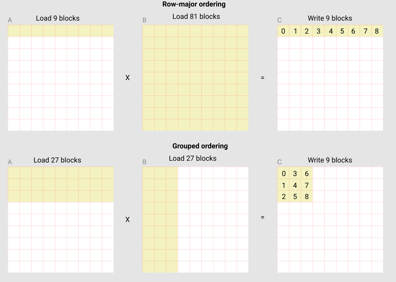
In reality, matrices are made an exact multiple of BLOCK_SIZE by padding with zeros. The algorithm is also adjusted to have different BLOCK_SIZE along each dimension. Each BLOCK_SIZE is chosen to optimally utilize the GPUs cache sizes. All of this is done behind the scenes by a compiler like TorchInductor.
Yet, these optimizations are generic and the compiler may miss certain optimizations you can leverage for your custom computational graph. In the next section, we shall dive deeper into the Triton programming language and explore cases where writing custom kernels can make the computations even faster.
Appendix
The following code was used as example for the demonstration of graph breaks.
import torch
from torch import _dynamo as torchdynamo
from typing import List

def custom_compiler(gm: torch.fx.GraphModule, example_inputs: List[torch.Tensor]):
    # PyTorch provides ability to define custom compilers.
    # Custom compiler should take input a graph module and return a callable.
    # We define a custom compiler that does nothing and returns the
    # forward method of the FX graph
    return gm.forward

# Our tensor function to compile
def leaky_relu(a):
    if a > 0:
        return a
    return 0.1 * a

if __name__ == "__main__":
    leaky_relu_compiled = torch.compile(leaky_relu, backend="inductor")
    y = leaky_relu_compiled(torch.randn((1,), requires_grad=True))
To obtain the FX graphs, code generated from FX graph using Torch operations, forward and backward code generated by AOTAutograd using aten opset and the original and modified Python bytecode, run the Python file using the collowing command.
TORCH_LOGS="dynamo,aot,bytecode" python triton/dynamo_debug.py
Additionally, TORCH_LOGS=”all” prints the entire process in detail.