
Multi-GPU Distributed Training
In the previous post, we used a single GPU to train a small, 117 million parameter model (GPT-2-small) with a batch size of 32 and a subset of optimizations -
- Asynchronous I/O.
- Four gradient accumulation steps.
- And torch.compile with default parameters.
In this post, we shall start with a 1.4 billion parameter model GPT2-large and progressively move on to even larger models.
First, let's define some terms for model sizes. For this, series, we shall call any model that can be trained using a reasonable configuration on a single GPU (standard GPUs these days range from 32 to 80 Gb) a small model.
In the next category are models whose entire parameters, optimizer states and stored gradients (which are only dependent on number of parameters) fit within a single GPU, yet they cannot be trained on one. This is because the peak memory consumed by the batch size and context length dependent activations during training leads to out-of-memory errors. We shall call such models, which can be trained on multiple GPUs without splitting the network, as large models.
Finally, for cases where the parameters, optimizer states and gradients do not fit within a single GPU, we need to split the model itself across multiple GPUs. We shall call this category massive models.
Today’s flagship models require clusters with thousands of GPUs to train a single model - distributing data, model and even context length across devices. For example, 16,000 H100 GPUs were used to train the largest Llama 3 model of 405 billion parameters. The data, context, model, optimizer states, gradients, individual transformer blocks and even individual layers were split across multiple GPUs to achieve the maximum compute utilization while minimizing inter-GPU communication and being within the constraints of available memory and network bandwidth. In this post, we shall learn to implement all of those techniques using at most a single node of 8 GPUs.
Large Models
First, let's try to train GPT2-large model with a batch size of 32 on our single L40S GPU (it is a popular GPU available on all cloud computing and AI platforms and has a memory of 48Gb). The 1.4 billion parameter model has the following configuration -
"n_layers": 48,
"num_heads": 25,
"embedding_dimension": 1600,
"vocabulary_size": 50257,
"context_length": 1024
Within the first micro-batch, we get an error -
torch.cuda.OutOfMemoryError: CUDA out of memory. Tried to allocate 200.00 MiB. GPU 0 has a total capacity of 44.53 GiB of which 137.25 MiB is free. Process 47091 has 44.39 GiB memory in use. Of the allocated memory 42.53 GiB is allocated by PyTorch, and 1.36 GiB is reserved by PyTorch but unallocated. If reserved but unallocated memory is large try setting PYTORCH_CUDA_ALLOC_CONF=expandable_segments:True to avoid fragmentation. See documentation for Memory Management (https://pytorch.org/docs/stable/notes/cuda.html#environment-variables)
This was expected as the model should consume about 69Gb according to the calculations in the previous post. In the case of batch size 32, out of the 69Gb peak,
- The parameters should take about 5.6 Gb (4 bytes per fp32 parameter times 1.4 billion parameters). Gradients should take an equal amount, and optimizer states for Adam should take twice of that (11.2 Gb). These are independent of the batch size.
- Majority of the rest of the approximately 46.6 Gb memory is occupied by batch size dependent activations (and a small portion by data and other buffers). By reducing the batch size, this peak memory consumption can be reduced proportionally.
Let's try with a batch size of 8. As seen below, the training run with batch size 8 fits comfortably within a single L40S 48Gb GPU. But a batch size of 8 is too small for training our model. Therefore, to achieve a batch size of 32, we would have to use four GPUs to split a batch of data.
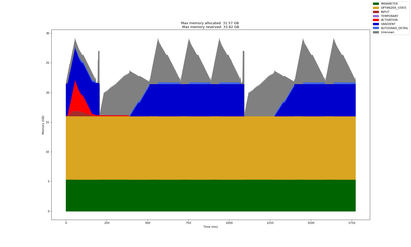
Also note that the profile chart for 1.4 billion parameter GPT looks quite different from the small models we trained in the previous post. Here, the parameters, gradients and optimizer states dominate the memory profile. This is important because as we grow our model size into the realm of massive models, the focus will be on distributing these efficiently across GPUs.
Data Parallelism
One way to achieve an effective batch size of 32 is to split a batch across the multiple GPUs. Each GPU has a copy of the full model's parameters for forward and backward pass. Each GPU computes gradients using its portion of the batch of data. The local gradients from all GPUs are collected and averaged. The averaged gradient is then applied to each copy of the model parameters.
This strategy will lead to exact same gradients (barring numerical issues) as a batch size of 32 on a single GPU. Since all copies of the model started from the same initial state and update with the same averaged gradient, they will have the exact same parameters at every step.
This paradigm is called Distributed Data Parallel (DDP) training. To perform DDP (and this applies to other distributed training strategies too), we need two things -
- A way to copy model parameters and data from CPU to individual GPUs.
- A way to communicate data (local gradients) between GPUs.
The first part, at least in DDP, is trivial with the .to() method. But the second part is tricky. First, the code responsible for communication should be aware of the network topology (for example, GPU 1 and 3 may not be directly connected in multi-node setups). Second, we need algorithms that communicate the required information efficiently to minimize data transfer latencies and network congestions in a given topology. For instance, in our case, every GPU needs local gradients from all other GPUs. If each local gradient is $P$ Mb in size, we need to communicate $P\times \left(P-1\right)$ Mb in a naive implementation of all-to-all data transfer (quadratic in the number of GPUs). Alternatively, we can use DeepSpeech's efficient ring all reduce algorithm. Discussion of inter-GPU communication primitives and algorithms is beyond the scope of this post. For detailed information, refer to this guide by PyTorch.
PyTorch provides convenient higher-level APIs for DDP training so that you do not have to worry about data transfers and distributed communication. Here is the code for using four GPUs to train GPT2-large with a batch size of 32. Each GPU processing a batch of 8 samples. Each batch of 8 is as usual further split into micro-batches of 2 for gradient accumulation.
import os, json, math, time
from datetime import datetime

import torch
import torch.distributed as dist
from torch.nn.parallel import DistributedDataParallel as DDP
from torch.utils.data import DataLoader, DistributedSampler
from torch.nn.functional import cross_entropy
from torch.optim import Adam

from torch.utils.tensorboard import SummaryWriter
from torch.profiler import profile

from trace_handler import trace_handler
from layers.model import EduLLM
from datasets.food_com_cc_cleaned.food_dot_com_recipes_dataset import FoodDotComRecipesDataset

# Constants
CONFIG_NAME = "gpt2"
CONFIG_FILE = f"./configs/{CONFIG_NAME}.json"
CHECKPOINT_FOLDER = "./checkpoints"
LOGS_FOLDER = "./logs"
PADDING_TOKEN_ID = 254
TIME_FORMAT_STR = "%b_%d_%H_%M_%S"

# Load config
with open(CONFIG_FILE, "r") as f:
    CONFIG = json.load(f)

# Enable TF32
torch.backends.cuda.matmul.allow_tf32 = True
torch.backends.cudnn.allow_tf32 = True


def setup_ddp():
    dist.init_process_group(backend='nccl')
    local_rank = int(os.environ['LOCAL_RANK'])
    torch.cuda.set_device(local_rank)
    return local_rank

def cleanup_ddp():
    dist.destroy_process_group()

def get_total_params(module: torch.nn.Module):
    return sum(p.numel() for p in module.parameters())


def train(local_rank):
    device = torch.device(f"cuda:{local_rank}")
    training_data = FoodDotComRecipesDataset("./datasets/food_com_cc_cleaned", split="train")
    sampler = DistributedSampler(training_data, shuffle=True)
    train_dataloader = DataLoader(training_data, batch_size=CONFIG["batch_size"],
                                  sampler=sampler, pin_memory=True, num_workers=2)

    model = EduLLM(
        n_layers=CONFIG["n_layers"],
        num_heads=CONFIG["num_heads"],
        embedding_dimension=CONFIG["embedding_dimension"],
        vocabulary_size=CONFIG["vocabulary_size"],
        context_length=CONFIG["context_length"],
    ).to(device)
    model = DDP(model, device_ids=[local_rank])
    optimizer = Adam(model.parameters(), lr=CONFIG["lr_fixed"])
    gradient_accumulation_steps = CONFIG["gradient_accumulation_steps"]

    with profile(
        activities=[torch.profiler.ProfilerActivity.CPU, torch.profiler.ProfilerActivity.CUDA],
        schedule=torch.profiler.schedule(wait=2 * gradient_accumulation_steps, warmup=gradient_accumulation_steps,
                                         active=2 * gradient_accumulation_steps, repeat=1),
        record_shapes=True,
        profile_memory=True,
        with_stack=True,
        on_trace_ready=trace_handler,
    ) as prof:
        for epoch in range(CONFIG["num_epochs"]):
            sampler.set_epoch(epoch)
            for batch, (inputs, targets) in enumerate(train_dataloader):
                micro_batch_size = inputs.shape[0] // gradient_accumulation_steps
                micro_batch_inputs = inputs[:micro_batch_size, :].to(device, non_blocking=True)
                micro_batch_targets = targets[:micro_batch_size, :, :].to(device, non_blocking=True)

                for micro_batch_step in range(1, gradient_accumulation_steps):
                    prof.step()
                    start, end = micro_batch_step * micro_batch_size, (micro_batch_step + 1) * micro_batch_size
                    next_inputs = inputs[start:end, :].to(device, non_blocking=True)
                    next_targets = targets[start:end, :, :].to(device, non_blocking=True)

                    preds = model(micro_batch_inputs, train=True)
                    loss = cross_entropy(
                        preds.view(-1, preds.size(-1)),
                        micro_batch_targets.view(-1),
                        ignore_index=PADDING_TOKEN_ID,
                        reduction="mean",
                    )
                    loss = loss / gradient_accumulation_steps
                    loss.backward()

                    micro_batch_inputs = next_inputs
                    micro_batch_targets = next_targets

                prof.step()
                preds = model(micro_batch_inputs, train=True)
                loss = cross_entropy(
                    preds.view(-1, preds.size(-1)),
                    micro_batch_targets.view(-1),
                    ignore_index=PADDING_TOKEN_ID,
                    reduction="mean",
                )
                loss = loss / gradient_accumulation_steps
                loss.backward()

                optimizer.step()
                optimizer.zero_grad(set_to_none=True)

if __name__ == "__main__":
    local_rank = setup_ddp()
    train(local_rank)
    cleanup_ddp()
To run the code, we need the torchrun module. The parameter nproc_per_node specifies the number of processes that will parallelly run the script (in this case train_ddp.py). The number should be less than or equal to the number of GPUs in the node as each process will operate on a single GPU. In our case, we have single node with four L40S GPUs and so we shall set this parameter to 4.
torchrun --nproc_per_node=4 train_ddp.py
Module torchrun will setup a distributed communications backend on every GPU, launch processes with your script on every GPU and provide environment variables for those processes to help them use the communication backend. For example, in above code, we have
local_rank = int(os.environ['LOCAL_RANK'])
which is used in the process to identify the GPU it is running on. This identifier is then used to transfer data and model from CPU to that GPU.
def train(local_rank):
    device = torch.device(f"cuda:{local_rank}")
    ...
    model = EduLLM(
        n_layers=CONFIG["n_layers"],
        num_heads=CONFIG["num_heads"],
        embedding_dimension=CONFIG["embedding_dimension"],
        vocabulary_size=CONFIG["vocabulary_size"],
        context_length=CONFIG["context_length"],
    ).to(device)
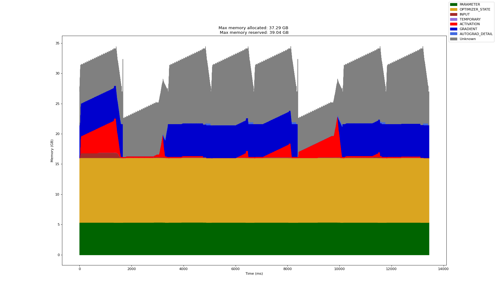
Here is the memory profile for one of the four GPUs during training. The peak memory usage on every GPU (which processes a batch of 8) is just 7 Gb higher compared to training with batch size 8 on single GPU. It is still within bounds of each GPUs capacity while achieving an effective batch size of 32!
Debugging Common Issues
Distributed training can introduce many issues not encountered in single GPU training. For instance, in the previous chart, note that the time taken for a batch of 8 samples on one of the GPUs in DDP is an order of magnitude higher (compared to training on a single GPU with batch size 8)!
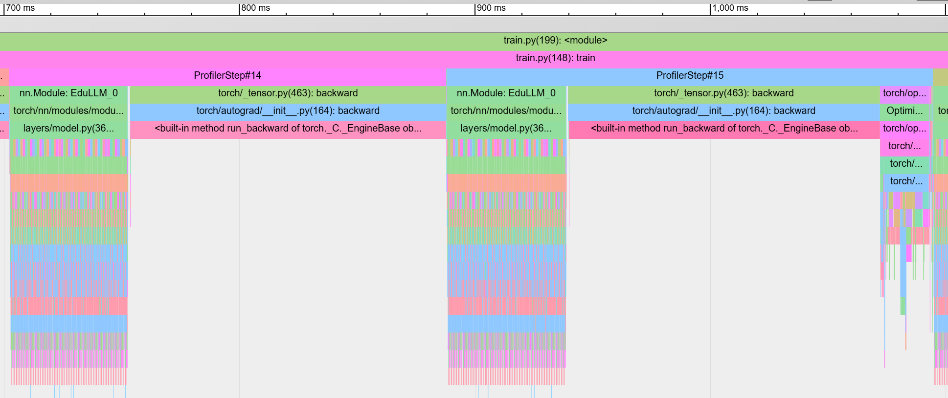
Let's investigate more by looking at the trace of one iteration in both cases. The following chart shows the trace of training with batch size 8 on a single GPU. The steps ProfilerStep#14 + ProfilerStep#15 (which constitute of forward and backward pass of two micro-batches followed by one optimizer run) takes a total of 396ms (187ms for #14 and 209ms for #15 which also includes the optimizer step).
On the other hand, the chart below shows the trace for one of the GPU processing a batch size of 8 in data parallelism paradigm. Here, ProfilerStep#14 (which constitute of forward and backward pass of two micro-batches) alone takes 1653ms! A 9x increase. Why are the forward and backward passes slower when using multiple GPUs? There is no inter-GPU communication during that phase. Let's dig deeper.
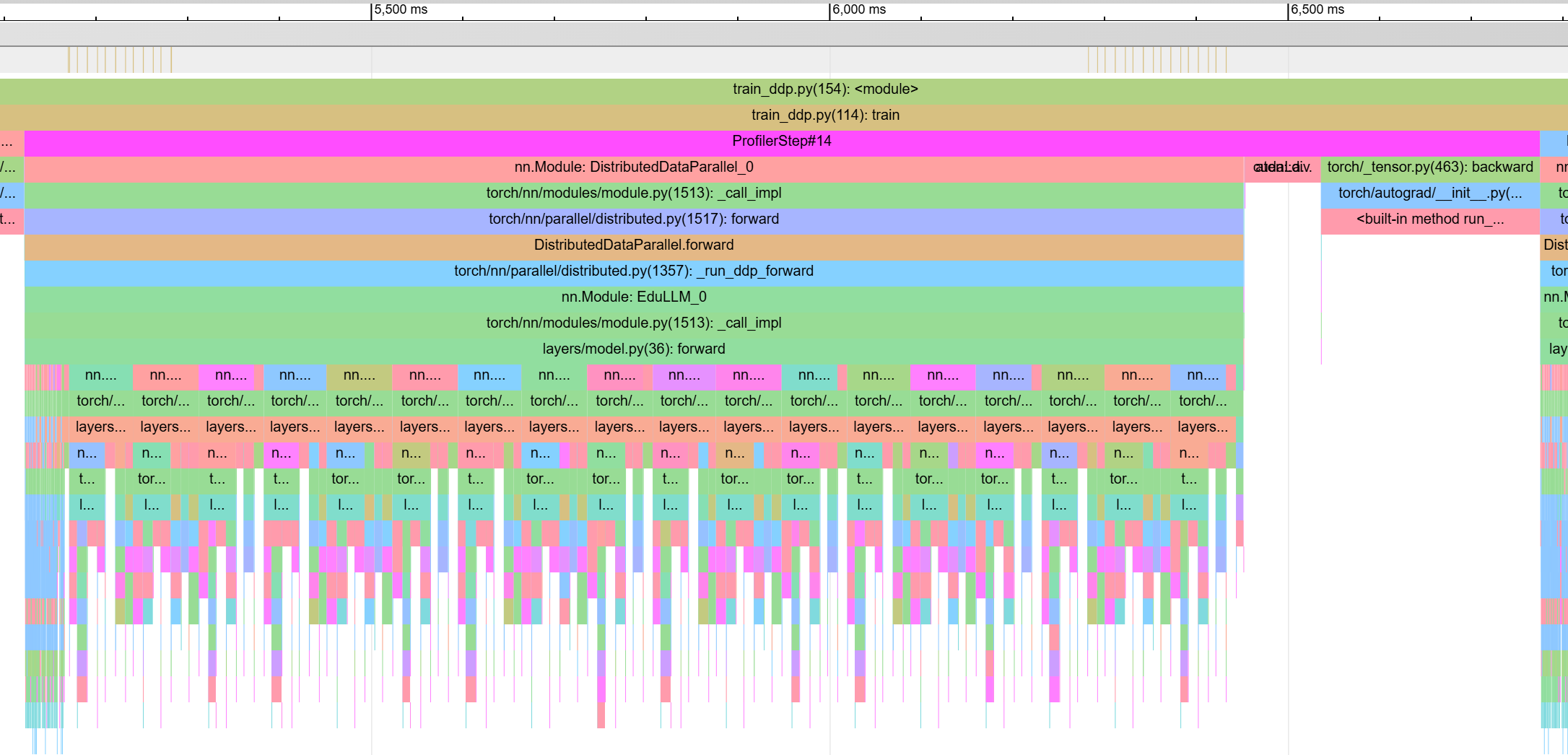
The chart below shows the zoomed in version of same step.
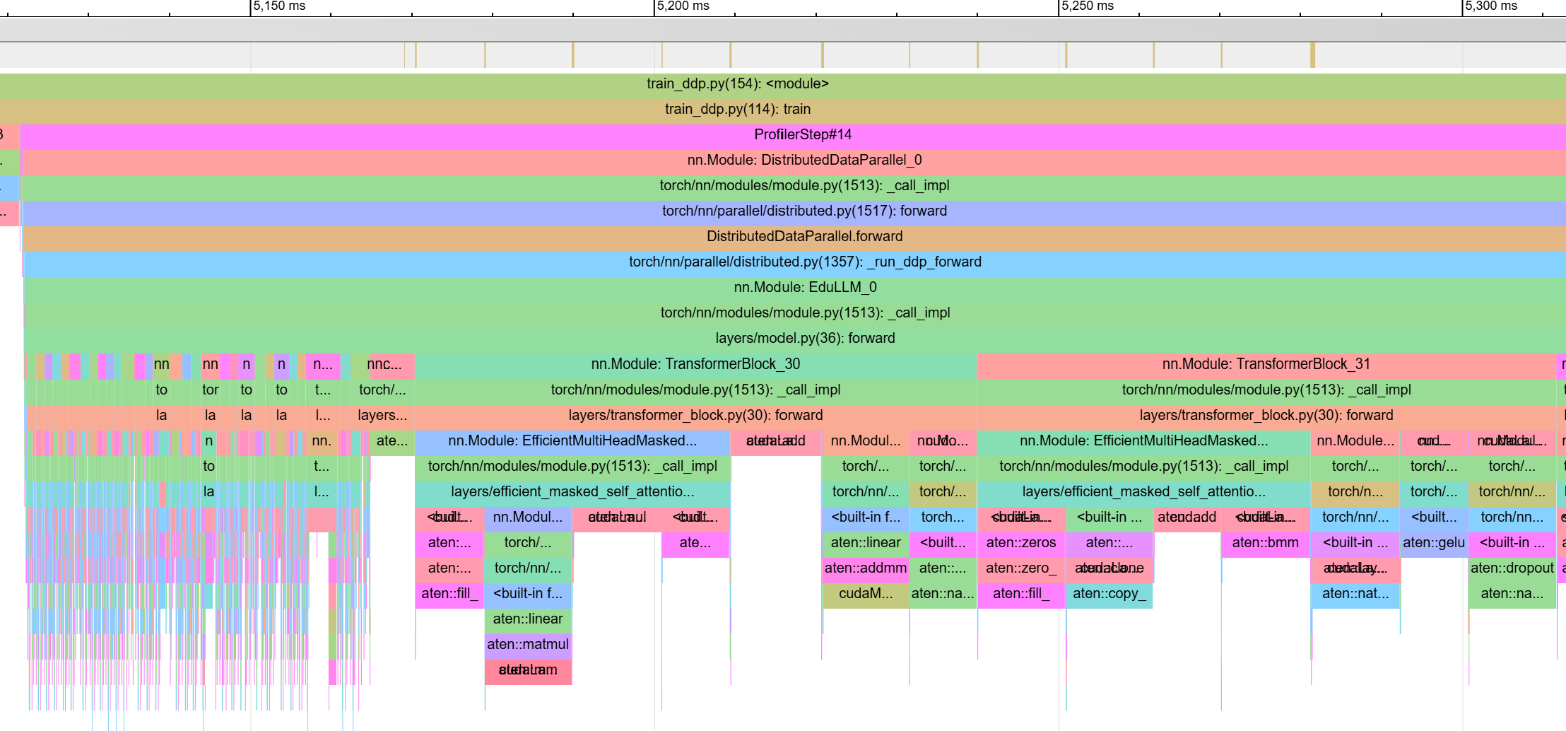
You can see that TransformerBlock_30 and onwards is taking lot more time compared to TransformerBlock_0 to TransformerBlock_29. Most of the time after TransformerBlock_30 is spent on cudaLaunchKernel step! This gives us the hint.
Note that even when we are using a multi-GPU setup for distributed training, we are still using a single node which means a single multi-core CPU and network interface. And it's the CPU that launches kernels on GPU. In this case the CPU is getting bottlenecked by launching many small kernels on the GPUs.
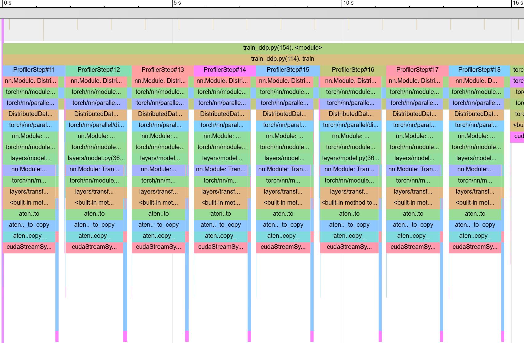
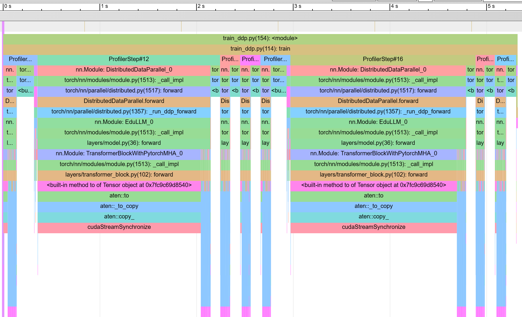
This is where, as shown in previous blog post, the efficiency of kernel fusion and PyTorch's built in MultiheadAttention can help us. By fusing the kernels within attention layer, there is less overhead of launching kernels as each kernel encompasses more operations. Below chart shows the trace from one of the four GPUs after switching to PyTorch MultiheadAttention in our model. The chart shows two batches with four micro batches each. You can see that all forward/backward passes (which are the tallest spikes) took equal times and if you zoom in further, you can see all transformer blocks took equal time. We have gotten rid of the kernel launch bottleneck.
Yet, even in this case, the runtime of 8 micro batches is approximately 15s compared to 2s for 8 micro batches on a single GPU. A majority of the time is spent on cudaStreamSynchronize within aten::copy_ step.
The fact that this is happening before every micro-batch's forward/backward pass gives us the hint. The DDP API in PyTorch will aggregate gradients from all GPUs after every call to backward. This means inter-GPU communication is happening after every micro-batch which is not what we want. With gradient accumulation, every GPU should locally collect gradients till all micro batches are exhausted. Local gradients should be collected and averaged only before the optimizer step. This can be achieved by the no_sync() context manager. The modified loop looks like the following with just a one line change.
for epoch in range(CONFIG["num_epochs"]):
    sampler.set_epoch(epoch)
    for batch, (inputs, targets) in enumerate(train_dataloader):
        micro_batch_size = inputs.shape[0] // gradient_accumulation_steps
        micro_batch_inputs = inputs[:micro_batch_size, :].to(device, non_blocking=True)
        micro_batch_targets = targets[:micro_batch_size, :, :].to(device, non_blocking=True)

        for micro_batch_step in range(1, gradient_accumulation_steps):
            prof.step()
            start, end = micro_batch_step * micro_batch_size, (micro_batch_step + 1) * micro_batch_size
            next_inputs = inputs[start:end, :].to(device, non_blocking=True)
            next_targets = targets[start:end, :, :].to(device, non_blocking=True)
            with model.no_sync(): # Do not sync between microbatches
                preds = model(micro_batch_inputs, train=True)
                loss = cross_entropy(
                    preds.view(-1, preds.size(-1)),
                    micro_batch_targets.view(-1),
                    ignore_index=PADDING_TOKEN_ID,
                    reduction="mean",
                )
                loss = loss / gradient_accumulation_steps
                loss.backward()

            micro_batch_inputs = next_inputs
            micro_batch_targets = next_targets

        prof.step()
        preds = model(micro_batch_inputs, train=True)
        loss = cross_entropy(
            preds.view(-1, preds.size(-1)),
            micro_batch_targets.view(-1),
            ignore_index=PADDING_TOKEN_ID,
            reduction="mean",
        )
        loss = loss / gradient_accumulation_steps
        loss.backward() # Sync between batches

        optimizer.step()
        optimizer.zero_grad(set_to_none=True)
The following chart shows the result of the fix. Now the 8 micro batches run in just 5s. The extra 3 seconds are spent on the two cudaStreamSynchronize after the two batches to accumulate gradients. Thats a small price to pay for the ability to train on larger batch sizes.
We now have a fast, distributed data parallel setup to train GPT2-large with batch size of 32!
Note that we use gradient accumulation to save on peak memory due to batch size dependent activations. But as models are growing larger, we see that it's the batch size independent parameters, gradients and optimizer states that take most of the memory. Moreover, gradient accumulation slows us down by having to run the micro-batches sequentially.
In the next section, we shall see an advanced version of data parallelism called Fully Sharded Data Parallelism (FSDP) that save memory by sharding (distributing) parameters, gradients and optimizer states across GPUs. With FSDP, we shall be able to train GPT2-large without gradient accumulation on 4 GPUs with the same effective batch size of 32.
Fully Sharded Data Parallelism
Note that, during the forward pass, every transformer layer has to run sequentially as each layer depends on the previous layer's output. But to execute a particular layer in forward pass, we do not need other layers of the model on the GPU memory.
For instance, every GPU does not need to store a full copy of the model parameters. The only requirement is that while executing forward pass of layer N on GPU X, all parameters of layer N must be present on GPU X. It does not matter if other layers of the model are not present on GPU X at that time.
Fully Sharded Data Parallelism (FSDP) is a variant of DDP where we partition and store model parameters (and gradients and optimizer states) across GPUs and only collect/discard them as and when required.
Let's say you have four GPUs. In FSDP, every weight matrix inside the model can be sharded (divided and distributed) such that each GPU only holds a fourth of the weight matrix. How you divide the matrix does not matter. Every GPU could hold a fourth of the total rows or a fourth of the total columns or any arbitrary distribution strategy. When the time comes to use that matrix during forward pass on GPU N,
- All shards of the matrix are collected from all GPUs onto GPU N.
- The complete matrix is used to perform computation and produce output.
- The shards of matrix that were pulled from other GPUs are dropped to reclaim memory.
While this is happening, rest of the matrices in the model remain sharded and therefore the sharded model only occupies a fourth of the total memory required for storing parameters (except for one matrix that is stored un-sharded while in use).
The same strategy can also be applied during backward pass where parts of a matrix are only collected before the backward pass and then discarded.
Also, such sharding strategy can also be applied to optimizer states, gradients and even activations. All of this is happening in combination with data parallelism.
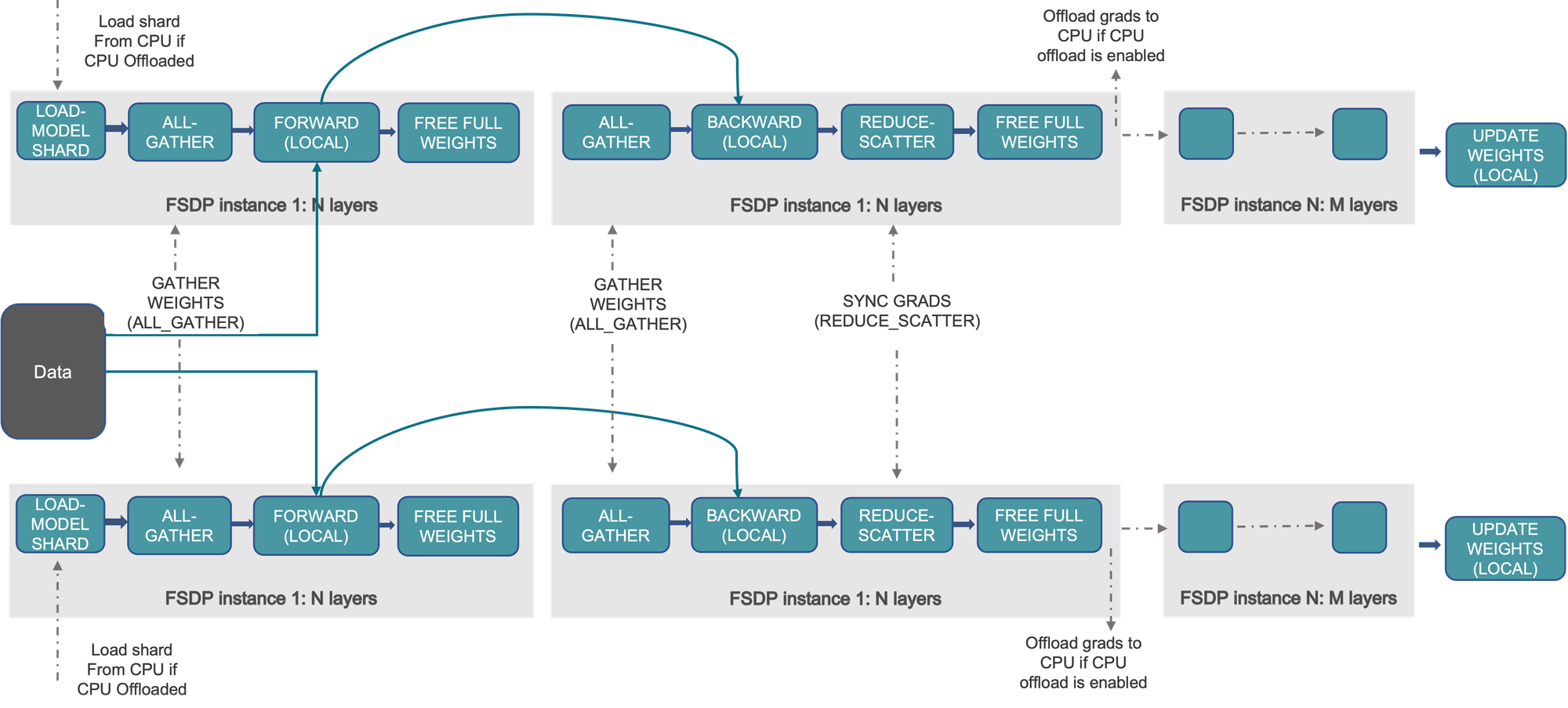
The following diagram from PyTorch docs shows the flow in FSDP.
FSDP is easy to implement with PyTorch FSDP2 API. After the model is initialized, you need to call
model = EduLLM(
    n_layers=CONFIG["n_layers"],
    num_heads=CONFIG["num_heads"],
    embedding_dimension=CONFIG["embedding_dimension"],
    vocabulary_size=CONFIG["vocabulary_size"],
    context_length=CONFIG["context_length"],
).to(device)
for layer in model.transformer:
    fully_shard(layer)
fully_shard(model)
Additionally, since we do not need gradient accumulation, we can simplify the training loop to the standard form
for epoch in range(CONFIG["num_epochs"]):
    sampler.set_epoch(epoch)
    for batch, (inputs, targets) in enumerate(train_dataloader):
        inputs.to(device, non_blocking=True)
        targets.to(device, non_blocking=True)
        preds = model(inputs, train=True)
        loss = cross_entropy(
            preds.view(-1, preds.size(-1)),
            targets.view(-1),
            ignore_index=PADDING_TOKEN_ID,
            reduction="mean",
        )
        loss.backward()
        optimizer.step()
The following chart shows the memory profile of one of the four GPUs while training 2 batches of 8 samples without gradient accumulation.
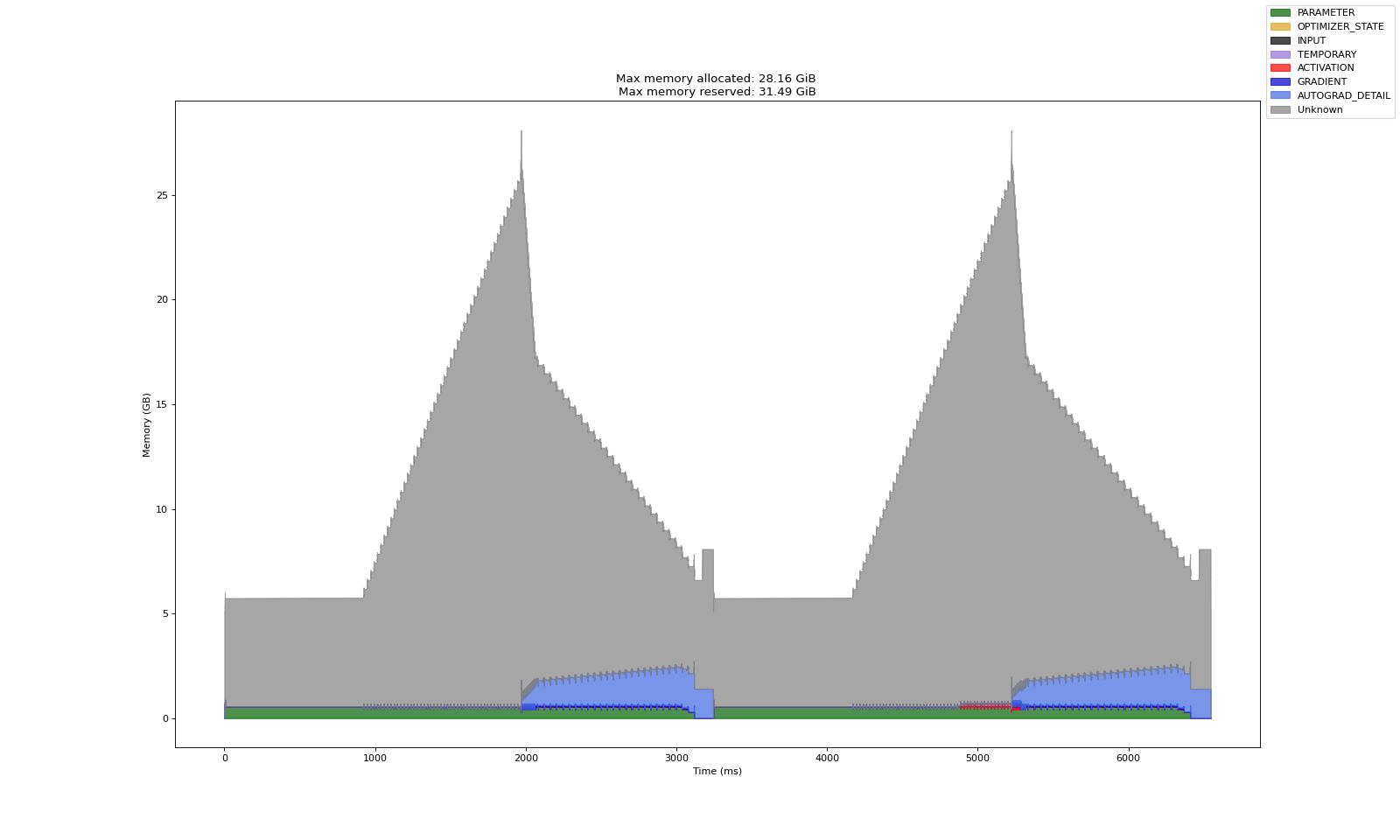
Note that memory occupied by parameters (as well as gradients and optimizer states not correctly attributed here) is about one fourth of the total in this case which allows us to not rely on sequential gradient accumulation. The time taken for 2 batches in this case was slightly higher that with DDP and gradient accumulation. But as model get larger and inter-GPU communication gets faster, FSDP will outperform sequential nature of gradient accumulation.
Model and Pipeline Parallelism
FSDP can be used to train large multi-billion parameter models on a cluster of GPUs. But it requires communication of all parameters from every GPU to every other GPU. Therefore, the data communicated between GPUs grows quadratically with model size and as model size increases to tens of billion parameters, this communication starts becoming a bottleneck.
Model parallelism is a different way of dividing a model across multiple GPUs while limiting the amount of inter-GPU communication. In model parallelism, a sequential model is divided into stages, and each GPU holds one stage of the model. For example, in a 12-layer transformer on a 4 GPU node, we can assign 3 layers to each GPU. But since each layer depends on previous layer's output, GPUs will be idle most of the time. For instance, while GPU 2 is processing layers 4-6, GPU 1, 3 and 4 are sitting idle.
Therefore, model parallelism is often used in a pipelined fashion and the resulting architecture is called pipeline parallelism. Let's consider that your model has 4 layers and we have a four GPU node. We distribute layers such that device 1 holds the first layer, device 2 holds the second, device 3 the third and final layer resides on device 4. We also divide a batch of data into 8 micro-batches but each GPU processes all the 8 micro-batches. The following chart shows the timeline of computation.
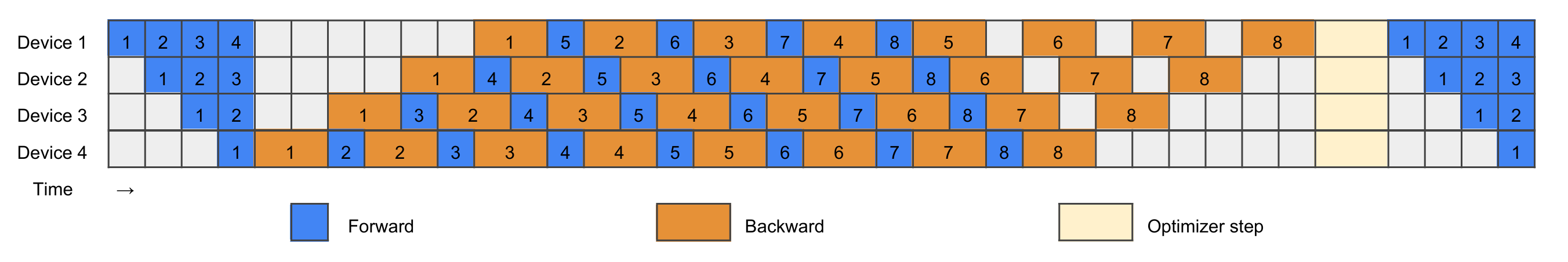
At timestep 1, device 1 (which holds the first layer) executes forward pass for micro-batch 1. At timestep 2, device 1 executes forward pass of micro-batch 2 while parallelly, device 2 executes the forward pass for micro-batch 1. At timestep 5, all devices have finished the forward pass of micro-batch 1 and device 4 (which holds the final layer) begins the backward pass of micro-batch 1. At timestep 7, final layer has finished the backward pass for micro-batch 1 and device 3 (which holds the third layer) can start the backward pass for micro-batch 1. Meanwhile, device 4 can finish the forward pass for micro-batch 2 through the last layer. And so on.
There are many things to note in this chart -
- First, the backward pass is shown to take twice the time of forward. This is because backward pass has to make more computations than forward - compute derivative of layer output w.r.t. layer parameters and w.r.t layer inputs.
- Second, the computation load (time taken for a forward or backward pass) is shown to be equally balanced across GPUs which is difficult to achieve.
- Third, the optimizer step has to be performed after all micro-batches have finished forward and backward passes through all layers.
- Finally, there are some timesteps where some GPUs are sitting idle. For example, devices 1, 2 and 3 at timestep 5. These empty regions in the chart are called pipeline bubbles.
Even though both FSDP and pipeline parallelism distribute the model across GPUs and solve the memory limitation, one requires higher communication while other suffers from pipeline bubbles. Popular distributed training helper libraries like DeepSpeed use intelligent interleaving of forward, backward and optimizer steps to minimize such bubbles. For example, this research paper introduces a pipelining scheme that results in zero bubbles!
An efficient pipeline parallelism scheme is quite difficult to implement with plain PyTorch and its distributed communications API. All optimization techniques we saw till DDP and FSDP did not require any model code change. But implementing efficient pipeline parallelism will require us to make pipeline parallelism specific code changes to the model. TorchTitan is one such project that has examples of implementing different parallelism strategies with PyTorch. In this tutorial, we shall use the DeepSpeed library which has a more convenient API for implementing all combinations of parallelism.
With DeepSpeed, we first need to modify our model code such that we can return a list of sequentially running modules. The modules in this list need not be nn.Module but anything that has a __call __() method defined. We will use this because our embedding layers are not sequential in nature. We define a to_layers() method that returns the list. DeepSpeed will automatically split this list across GPUs according to our configurations.
class EduLLMPP(nn.Module):
    def __init__(self, n_layers: int, num_heads: int, embedding_dimension: int, vocabulary_size: int, context_length: int):
        super().__init__()
        self.token_embedding = nn.Embedding(vocabulary_size, embedding_dimension)
        self.positional_embedding = nn.Embedding(context_length, embedding_dimension)
        self.embedding_layers = [lambda x: self.embedding_layer(x)]

        self.transformer_layers = [
            TransformerBlockWithPytorchMHA(num_heads, embedding_dimension, True) for _ in range(n_layers)
        ]

        ln = nn.LayerNorm(embedding_dimension)
        head = nn.Linear(embedding_dimension, vocabulary_size, bias=False)
        self.projection_layers = [ln, head]

    def embedding_layer(self, x):
        device = x.device
        [batch_size, context_length] = x.shape
        positions = torch.arange(0, context_length, step=1, device=device, requires_grad=False) # [context_length]
        pe = self.positional_embedding(positions) # [batch_size, context_length, embedding_dimension]
        te = self.token_embedding(x) # [batch_size, context_length, embedding_dimension]
        return te + pe # [batch_size, context_length, embedding_dimension]

    def to_layers(self):
        layers = [
            *self.embedding_layers,
            *self.transformer_layers,
            *self.projection_layers
        ]
        return layers
Then the training loop looks like the following piece of code
import torch, json, os
from torch.nn.functional import cross_entropy
import deepspeed
from deepspeed.pipe import PipelineModule
from layers.model import EduLLMPP
from datasets.food_com_cc_cleaned.food_dot_com_recipes_dataset import (
    FoodDotComRecipesDataset,
)

# Constants
CONFIG_NAME = "gpt2"
CONFIG_FILE = f"./configs/{CONFIG_NAME}.json"
CHECKPOINT_FOLDER = "./checkpoints"
LOGS_FOLDER = "./logs"
PADDING_TOKEN_ID = 254
TIME_FORMAT_STR = "%b_%d_%H_%M_%S"

# Load config
with open(CONFIG_FILE, "r") as f:
    CONFIG = json.load(f)


def loss_fn(output, labels):
    return cross_entropy(
        output.view(-1, output.size(-1)),
        labels.view(-1),
        ignore_index=PADDING_TOKEN_ID,
        reduction="mean",
    )


class DeepSpeedArgs:
    def __init__(self, local_rank):
        self.local_rank = local_rank


def train():
    args = DeepSpeedArgs(local_rank=int(os.environ.get("LOCAL_RANK")))

    training_data = FoodDotComRecipesDataset(
        "./datasets/food_com_cc_cleaned", split="train"
    )

    model = EduLLMPP(
        n_layers=CONFIG["n_layers"],
        num_heads=CONFIG["num_heads"],
        embedding_dimension=CONFIG["embedding_dimension"],
        vocabulary_size=CONFIG["vocabulary_size"],
        context_length=CONFIG["context_length"],
    )

    model = PipelineModule(
        layers=model.to_layers(),
        num_stages=4,
        loss_fn=loss_fn,
        partition_method="uniform",
        activation_checkpoint_interval=0,
    )

    model_engine, _, _, _ = deepspeed.initialize(
        args=args,
        model=model,
        model_parameters=[p for p in model.parameters() if p.requires_grad],
        training_data=training_data,
        config="ds_config.json",
    )

    for epoch in range(1):  # Train for 10 epochs as an example
        for step in range(len(training_data)):
            loss = model_engine.train_batch()


if __name__ == "__main__":
    deepspeed.init_distributed()  # Similar to init_process_group in DDP and sets the env variable LOCAL_RANK
    train()
Note that we did not create an optimizer here. DeepSpeed library relies heavily on configurations specified via a JSON config file. In our case, we create a ds_config.json and pass it to deepspeed.initialize for it to configure the model engine.
Also note that the training loop is quite simple with just a model_engine.train_batch(). The model engine has access to loss function and training dataset and does all the heavy lifting of distributed data loading behind the scenes for you.
To replicate our previous training configurations, the ds_config.json looks as follows.
{
    "train_batch_size": 32,
    "train_micro_batch_size_per_gpu": 8,
    "gradient_accumulation_steps": 4,
    "optimizer": {
        "type": "Adam",
        "params": {
            "lr": 0.0005
        }
    },
    "fp16": {
        "enabled": false
    },
    "zero_optimization": {
        "stage": 0
    }
}
The zero_optimization field holds all the configuration for implementing FSDP using ZeRO. But ZeRO stage 2 (optimizer + gradient partitioning) and 3 (optimizer + gradient + parameter partitioning) are not supported with pipeline parallelism in DeepSpeed. Therefore, we disable FSDP by setting ZeRO stage to 0. Rest of the settings are same as previous training runs. There are a lot more configurations you can specify via this file. Read DeepSpeed docs for full details.
To execute, you run
deepspeed --num_gpus=4 train_pp.py
and DeepSpeed will handle the entire schedule for you. DeepSpeed uses simple pipeline parallel schedule which will be prone to bubbles. Efficient implementation is beyond the scope of this tutorial.
Pipeline parallelism requires us to make significant code change. Moreover, we need to test multiple configurations to find the schedule with minimal pipeline bubbles. In contrast, FSDP was quite easy to use and works out of the box. Therefore, FSDP is quite helpful to get started quickly, especially in fine-tuning scenarios where you may not want to change model code. Both can also be used together too as we shall learn in multi-dimensional parallelism section later.
If you have access to a lot of GPUs, you technically do not need pipeline parallelism. FSDP, in combination with activation checkpointing will allow you to train even multi-billion parameter models without much code change. This is especially true for fine tuning scenarios where your compute hours are significantly less. Additionally, CPU offloading is a technique that can let you train even trillion parameter models using just FSDP and activation checkpointing.
Tensor Parallelism
As you keep scaling, there comes a point where large tensors will not fit within memory of a single GPU. At this point, the only way forward is to split individual tensors across multiple GPUs. This approach is known as tensor parallelism.
Tensor parallelism is not available out of the box with popular deep learning libraries. Instead, you will have to write custom modules that communicate with other GPUs at appropriate times in the forward and backward methods.
There are multiple ways to split a model across GPUs. Let’s look at an approach from Megatron-LM. Let’s look at a simple multi-layer perceptron (assume that bias, if required, is included by appending a column of ones to $X$).
$$ y = \text{ReLU}(XA) $$
here $A$ is a $N\times M$ sized matrix, $X$ is a $B\times N$ and $b$ is a $M\times 1$ vector. The result $y$ is a $B\times M$ matrix. One way to split the computation is by dividing columns of $X$ and rows of $A$. For instance, in case of two GPUs, we can divide columns of $X$ into $X_1$ and $X_2$ where both are $B\times N/2$ and divide rows of $A$ into $A_1$ and $A_2$ where both are $N/2\times M$. Then distribute $X_1$ and $A_1$ to one GPU and $X_2$ and $A_2$ to the other. To get back $XA$, we perform an all-reduce communication operation where all GPUs get a sum of $X_iA_i$ across all GPUs.
$$ X = [X_1, X_2] \\ A = \begin{bmatrix}A_1 \\ A_2 \end{bmatrix} , \\ XA = X_1A_1 + X_2A_2 $$
The all reduce operation is necessary before the $\text{ReLU}$ operation as
$$ \text{ReLU}(X_1A_1 + X_2A_2) \neq \text{ReLU}(X_1A_1) + \text{ReLU}(X_2A_2) $$
Another way we could split the inputs is by splitting columns of $A$ into $A_1$ and $A_2$ where both are size $N\times M/2$. Now, we can distribute $X$ and $A_1$ to one GPU and $X$ and $A_2$ to the other. Then,
$$ XA = [XA_1, XA_2], \\\\ \text{ReLU}(XA) = [\text{ReLU}(XA_1), \text{ReLU}(XA_2)] $$
Note that in this case, we did not require an all-reduce operation before the $\text{ReLU}$ activation.
The following figure from the 405 billion parameter Llama 3 paper shows how a cluster of GPUs are used to implement four-dimensional parallelism FSDP (shown as DP), Pipeline Parallelism (PP), Context Parallelism (CP) and Tensor Parallelism (TP). Such multi-dimensional parallelism is only used for massive models during pre-training stage where latency is also important.
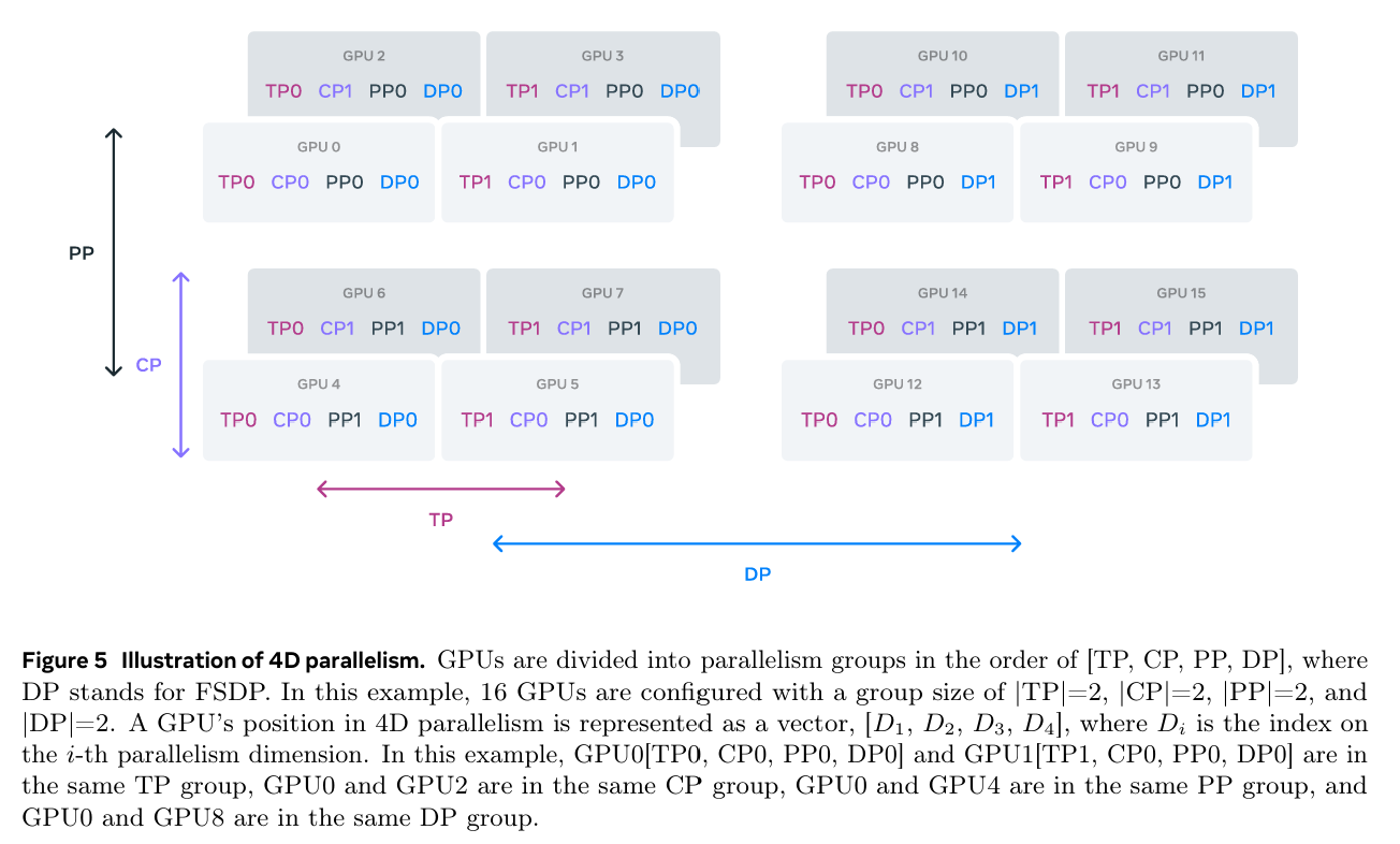
In most cases where the amount of training is low (for example in finetuning) FSDP with gradient checkpointing and CPU offloading should be sufficient for even a trillion-parameter model.