
Optimizing the Model Architecture
In the previous post, we saw how to optimize a generic training loop for large deep learning models. In this post, we shall implement a GPT-style decoder-only transformer model (most common large language model architecture) and explore some model architecture specific optimizations.
Although Large Language Models (LLMs) come with millions or even billions of parameters and exceptional natural language generation capabilities, their model architecture isn’t as complex as it might seem. Most popular LLMs use a model architecture known as Transformer. A Transformer is really just a combination of a few attention layers (specifically, self-attention layers for GPT-like decoder-only models), some normalization layers (like batch normalization and layer normalization), few multi-layer perceptrons and some residual connections. That’s all there is to it. The paper that introduced the Transformer family of architectures was aptly named “Attention Is All You Need”.
The same attention layer is also the bottleneck for memory and compute efficiency of transformers. Therefore, in this post, a disproportionate amount of attention will be given to optimizing them.
Model Architecture
Let’s start by implementing the traditional GPT style decoder only transformer architecture. We shall name this model EduLLM. In this initial implementation, we shall focus on readability and then, like previous section, optimize the architecture step by step.
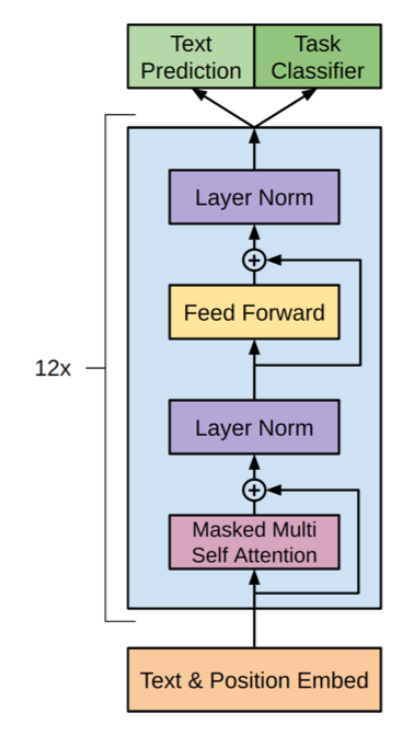
At a high level, the decoder looks like the accompanying diagram taken from the original GPT paper. It shows learnt text and positional embeddings followed by a stack of 12 blocks called the transformer layers. Each transformer block consists of a couple of layer normalization layers, a multi-layer perceptron and a masked multi-head self-attention. The block also has some residual connections.
The GPT 2 paper modifies this architecture by moving the layer normalization to the beginning of the transformer block and adding another layer normalization layer after the last transformer block. In this post, we shall be following those modifications.
Let’s start building in a top-down manner by first defining the model EduLLM comprising of embedding layers, stack of transformer blocks and final projection layers. We shall then define the transformer block, and then the masked multi-head attention layers. The inputs to the model are number of transformer layers, number of attention heads for multi headed attention, embedding dimension and vocabulary size.
import torch
from torch import nn
from layers.transformer_block import TransformerBlock

class EduLLM(nn.Module):
    def __init__(self, n_layers: int, num_heads: int, embedding_dimension: int, vocabulary_size: int, context_length: int):
        super().__init__()
        # Learnt token embeddings.
        self.token_embedding = nn.Embedding(vocabulary_size, embedding_dimension)
        # Learnt positional embeddings.
        self.positional_embedding = nn.Embedding(context_length, embedding_dimension)
        # Sequence layers of transformer blocks.
        self.transformer = nn.ModuleList(
            [TransformerBlock(num_heads, embedding_dimension, True)
            for _ in range(n_layers)])
        # Final layer normalisation.
        self.ln = nn.LayerNorm(embedding_dimension)
        # Projection layer to map embeddings to vocabulary size.
        self.head = nn.Linear(embedding_dimension, vocabulary_size, bias=False)
        # Tie token embedding and final projection layer weights.
        self.token_embedding.weight = self.head.weight
        # Recursively apply weight initialization.
        self.apply(self._initialize_weights)

    def forward(self, x, train: bool = True):
        [batch_size, context_length] = x.shape
        # Create positions array on same device as input tensor
        device = x.device
        positions = torch.arange(0, context_length, step=1, device=device, requires_grad=False) # [context_length]
        pe = self.positional_embedding(positions) # [batch_size, context_length, embedding_dimension]
        te = self.token_embedding(x) # [batch_size, context_length, embedding_dimension]
        x = te + pe # [batch_size, context_length, embedding_dimension]
        for transformer_block in self.transformer:
            x = transformer_block(x, train) # [batch_size, context_length, embedding_dimension]
        x = self.ln(x) # [batch_size, context_length, embedding_dimension]
        x = self.head(x) # [batch_size, context_length, vocabulary_size]
        return x

    def _initialize_weights(self, module):
        if isinstance(module, nn.Linear):
            nn.init.normal_(module.weight, mean=0.0, std=0.02)
            # Some linear layers do not have bias.
            # For example embeddings and head.
            if module.bias is not None:
                nn.init.zeros_(module.bias)
We will define TransformerBlock in the next section. Comments show the output shapes after each transformation in the forward method. Some things to note here are -
- The inputs to positional embedding layer (just a fixed sequence of numbers from 0 to
context_length) must be created on the same device as other tensors and should not require gradients as these are not parameters to the model. - The projection layer should not have a bias term.
- The
forwardmethod accepts Boolean parameter train that indicates whether to use dropout or not inside transformer block. Dropout is not used during inference. - The token embedding weight matrix of shape
[vocabulary_size, embedding_dimension]is shared with head projection layer weight matrix of shape[embedding_dimension, vocabulary_size]. The technique reduces the number of parameters without compromising on the quality. Note that theself.token_embedding.weight.shapeis[vocabulary_size, embedding_dimensionandself.head.weight.shapetoo is[vocabulary_size, embedding_dimension](in PyTorch, the Linear layer transposes its weight matrix before batch multiplying with its inputs: $y = xA^T + b$). Therefore, we can simply point one to the other asself.token_embedding.weight = self.head.weight. For more details, refer to an official example of weight tying used to tie encoder and decoder weights. - The default PyTorch constructor for
nn.Linearinitializes weights as uniform random numbers between a range that depends on shape of input. To recursively apply a different weight initialization strategy, we first define a function that accepts a module and initializes its weights according to the desired strategy. Then in the model’s constructor, we usenn.Module's apply method to apply this function recursively to all sub-modules starting fromEduLLM.
Transformer Block
The following code shows a single transformer block. The inputs to the transformer block are either the embedded sequence or outputs of previous transformer block. The inputs and outputs are of shape [batch_size, context_length, embedding_dimension].
import torch
from torch import nn
from layers.masked_self_attention import MultiHeadMaskedSelfAttention

class TransformerBlock(nn.Module):
    def __init__(self, num_heads: int, embedding_dimension: int, causal: bool = True):
        super().__init__()
        self.ln1 = nn.LayerNorm(embedding_dimension)
        self.attention = MultiHeadMaskedSelfAttention(num_heads, embedding_dimension, causal)
        self.attention_dropout = nn.Dropout(0.1)
        self.ln2 = nn.LayerNorm(embedding_dimension)
        self.linear = nn.Linear(embedding_dimension, 4 * embedding_dimension)
        self.act = nn.GELU()
        self.projection = nn.Linear(4 * embedding_dimension, embedding_dimension)
        self.projection_dropout = nn.Dropout(0.1)

    def forward(self, x, train: bool = True):
        # Layer normalisation
        y = self.ln1(x) # [batch_size, context_length, embedding_dimension]
        # Multi headed attention
        y = self.attention(y) # [batch_size, context_length, embedding_dimension]
        # Dropout
        if train:
            y = self.attention_dropout(y) # [batch_size, context_length, embedding_dimension]
        # Residual connection
        y = y + x # [batch_size, context_length, embedding_dimension]
        # Layer normalisation
        z = self.ln2(y) # [batch_size, context_length, embedding_dimension]
        # Multi layer perceptron
        z = self.linear(z) # [batch_size, context_length, embedding_dimension * 4]
        z = self.act(z) # [batch_size, context_length, embedding_dimension * 4]
        z = self.projection(z) # [batch_size, context_length, embedding_dimension]
        # Dropout
        if train:
            z = self.projection_dropout(z) # [batch_size, context_length, embedding_dimension]
        # Residual connection
        return y + z # [batch_size, context_length, embedding_dimension]
The comments show the output shapes after every transformation.
Multi-Head Self Attention Layer
Multi-head attention is described in the popular paper Attention is All You Need. For demonstration purposes, we shall create a MultiHeadMaskedSelfAttention module that holds num_heads independent individual attention layers (MaskedSelfAttention) that run sequentially. We shall later see a way to optimize this part.
MultiHeadMaskedSelfAttention creates multiple instances of MaskedSelfAttention with input dimension as embedding_dimension and output dimension as embedding_dimension / num_heads. Note that embedding_dimension should be an integral multiple of num_heads so that the outputs of individual heads can be concatenated back to return exactly embedding_dimension sized intermediate outputs.
import torch
from torch import nn

class MultiHeadMaskedSelfAttention(nn.Module):
    def __init__(self, num_heads: int, embedding_dimension: int, causal: bool = True):
        super().__init__()
        if embedding_dimension <= 0 and embedding_dimension % num_heads != 0:
            throw("hidden_dimension should be a multiple of num_heads")
        self.heads = nn.ModuleList(
            [MaskedSelfAttention(embedding_dimension, embedding_dimension // num_heads, causal) for _ in range(num_heads)])
    def forward(self, x):
        # x has shape [batch_size, context_length, embedding_dimension]
        attentions = [msa(x) for msa in self.heads] # A list of elements of shape [batch_size, context_length, embedding_dimension // num_heads]
        attention = torch.concatenate(attentions, dim=-1) # [batch_size, context_length, embedding_dimension]
        return attention
Having established the higher-level architecture, we now focus on the crux of the transformer architecture — the attention layer (named MaskedSelfAttention in this case).
Attention Layer
Broadly, learning with sequential data can be categorized into three major groups -
- Masked sequence learning: predicting tokens at masked positions based on rest of the tokens.
- Next token prediction : predicting next token based on a sequence of past tokens (of same vocabulary)
- Sequence to sequence translation : predicting next token based on a sequence of past tokens (of same vocabulary) and a reference sequence of tokens (of same or different vocabulary)
All three tasks can be accomplished with Transformer based models but the distinction is important because they differ in the type of attention layer used.
An attention layer works like a simple key-value table. For a given query, the table returns the weighted average of values where weights are proportional to the similarity between the query and keys. Note the difference between this table and a standard dictionary data structure. In an attention layer, even if you pass a query that is exactly equal to a key in the table, you wont get the exact associated value of the key. Values of other nearby keys will also play a role in the result.
In attention layer, the query, keys and values are all fixed sized vectors. The similarity of a query to all keys is computed using the dot product between every query-key pair. If there are K keys in the table, you get a vector of K scores for one query (1 scalar dot product between one query vector and each key vector). These K scores are normalized using a softmax function to get a K-sized attention vector of positive values that sum to 1. The attention vector can then be used to return a weighted average of L value vectors.
In the context of deep learning, we use a learnable attention layer. Which means, queries, keys and values are not direct tokens from the sequence but rather generated using a linear transformation applied to those tokens. The parameters of this transformation are learnt during training.
Let's implement the self-attention layer with PyTorch. All types of attention layers are built into the torch.nnmodule but implementing them using basic blocks will help us understand, debug and customize the transformations even better.
import torch
from torch import nn

class MaskedSelfAttention(nn.Module):
    def __init__(self, input_dimension: int, output_dimension: int, causal: bool = True):
        super().__init__()
        # Qeury, key and value projection layers
        self.wq = nn.Linear(input_dimension, output_dimension, bias=False)
        self.wk = nn.Linear(input_dimension, output_dimension, bias=False)
        self.wv = nn.Linear(input_dimension, output_dimension, bias=False)
        # Single non-trainable constant
        self.score_normalisation_factor = 1.0 / output_dimension
        # Softmax such that every row sums to 1
        self.softmax = nn.Softmax(dim=-1)
        # If using causal attention, a query cannot attend to
        # keys at future positions in the sequence
        self.causal = causal
    def forward(self, x):
        [batch_size, context_length, input_dimension] = x.shape
        # We create 2 new non-trainable matrices (additive_mask, causal_mask) at runtime
        # inside this function. We need to specify which device to create them on.
        device = x.device
        # Causal additive mask is constant and same for all samples
        with torch.no_grad():
            additive_mask = torch.zeros((context_length, context_length), device=device) # [context_length, context_length]
            if self.causal:
                additive_mask = torch.triu(
                    torch.full((context_length, context_length), float('-inf'), device=device),
                    diagonal=1) # [context_length, context_length]
        query = self.wq(x) # [batch_size, context_length, output_dimension]
        key = self.wk(x) # [batch_size, context_length, output_dimension]
        value = self.wv(x) # [batch_size, context_length, output_dimension]
        key_transpose = torch.transpose(key, 1, 2) # [batch_size, output_dimension, context_length]
        scores = torch.bmm(query, key_transpose) # [batch_size, context_length, context_length]
        masked_scores = scores + additive_mask # additive_mask is broadcasted to [batch_size, context_length, context_length]
        normalised_scores = masked_scores / self.score_normalisation_factor # [batch_size, context_length, context_length]
        attention_probabilities = self.softmax(normalised_scores) # [batch_size, context_length, context_length] where each row sums to 1.0
        self_attention = torch.bmm(attention_probabilities, value) # [batch_size, context_length, output_dimension]
        return self_attention
Profiling
With the model architecture setup, lets profile the forward pass. Below chart is the zoomed in version of ProfilerStep#6 from previous post. The view is zoomed in to just the forward pass (all operations shown are part of nn.Module: EduLLM_0 on level 4).
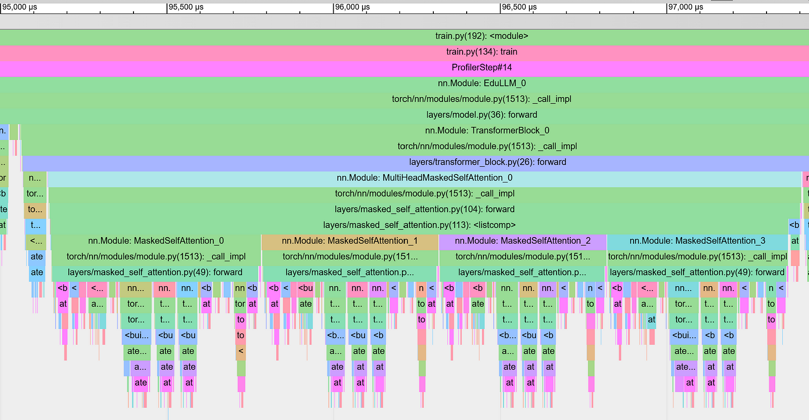
The time taken to run MultiHeadMaskedSelfAttention of one transformer block (TransformerBlock_0) is 2.261ms. One clearly visible inefficiency is the part where the four attention heads (nn.Module: MaskedSelfAttention) run sequentially. So let’s modify that to build a parallel multi-head attention.
import torch
from torch import nn

class EfficientMultiHeadMaskedSelfAttention(nn.Module):
    def __init__(
        self,
        num_heads: int,
        embedding_dimension: int,
        causal: bool = True
    ):
        super().__init__()
        assert embedding_dimension % num_heads == 0
        self.num_heads = num_heads
        self.wqkv = nn.Linear(embedding_dimension, 3 * embedding_dimension, bias=False)
        self.score_normalisation_factor = 1.0 / self.head_dimension
        self.softmax = nn.Softmax(dim=-1)
        self.causal = causal

    def forward(self, x):
        [batch_size, context_length, input_dimension] = x.shape
        device = x.device
        with torch.no_grad():
            additive_mask = torch.zeros(
                (context_length, context_length), device=device
            )
            if self.causal:
                additive_mask = torch.triu(
                    torch.full(
                        (context_length, context_length),
                        float("-inf"),
                        device=device,
                    ),
                    diagonal=1,
                )
        qkv = self.wqkv(x).view(
            (batch_size, context_length, self.num_heads, -1)
        )  # [batch_size, context_length, num_heads, 3*head_dimension]
        qkv = qkv.permute(
            (0, 2, 1, 3)
        )  # [batch_size, num_heads, context_length, 3*head_dimension]
        qkv = qkv.reshape(
            (batch_size * self.num_heads, context_length, -1)
        )  # [batch_size*num_heads, context_length, 3*head_dimension]
        query = qkv[:, :, : self.head_dimension]
        key = qkv[:, :, self.head_dimension : 2 * self.head_dimension]
        value = qkv[:, :, 2 * self.head_dimension :]
        key_transpose = torch.transpose(
            key, 1, 2
        )  # [batch_size*num_heads, head_dimension, context_length]
        scores = torch.bmm(
            query, key_transpose
        )  # [batch_size*num_heads, context_length, context_length]
        masked_scores = scores + additive_mask
        normalised_scores = (
            masked_scores / self.score_normalisation_factor
        )  # [batch_size*num_heads, context_length, context_length]
        attention_probabilities = self.softmax(
            normalised_scores
        )  # [batch_size*num_heads, context_length, context_length] where each row sums to 1.0
        self_attention = torch.bmm(attention_probabilities, value)
        return (
            self_attention.view((batch_size, self.num_heads, context_length, -1))
            .permute((0, 2, 1, 3))
            .reshape((batch_size, context_length, -1))
        )
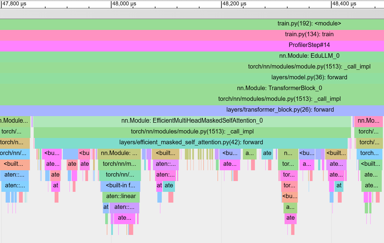
The chart below shows the zoomed in trace of EfficientMultiHeadMaskedSelfAttention within same layer (TransformerBlock_0). Note that the wall clock time of EfficientMultiHeadMaskedSelfAttention has dropped to 0.578ms!
The charts below show the effect of the modification on the overall training loop. The total training time for eight micro batches drops to half! With sequential MultiHeadMaskedSelfAttention based transformer block, it took ~250ms. While with parallel EfficientMultiHeadMaskedSelfAttention based transformer block, it took ~125ms.
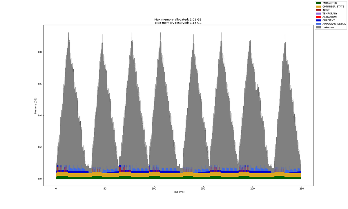
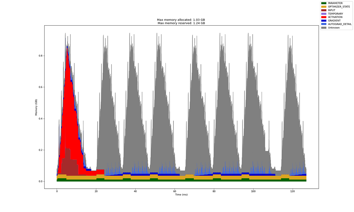
Note that (for reasons unknown) the profiler is not attributing memory correctly and often activation memory is attributed to other category. So, ignore the red vs. gray colors — both correspond to activation memory.
All the optimizations we explored till now had practically no effect on the final quality of the trained model (therefore we did not consider that as a factor). These were just engineering tricks and the model computes the same equations with same numbers.
But at this point, we shall explore some architectural changes that will allow us to be even more memory and compute efficient. These architectural changes will affect the model’s computation graph and should be evaluated by training the model and evaluating its quality too.
These architectural changes fall into two broad categories - sparsity and sharing
- Sparsity: In this technique, only a fraction of the network parameters contributes to the final loss. The subset of weights that will be used depends on the inputs and the current weight values themselves. Examples of this technique are Sparse Attention and Mixture of Experts (MoE). Many flagship massive LLMs use MoE to increase the model's "capacity" without affecting its latency. Since optimizer states don't have to be stored for all parameters, it also helps reduce memory consumption. Other example are approaches (like Linformer) that assumes large matrices (such as attention scores) are dominated by a few values and can therefore be decomposed into product of smaller matrices also fall in this category.
- Sharing: In this technique, different projection layers are made to share common weight matrices. We have already seen an example of this where we shared the weights for embeddings and final projection layer. Other examples are query-key weight sharing and Grouped Query Attention (GQA). GQA is also popularly used by many modern LLMs.
Let's implement some of these to see their effectiveness.
Query-Key Weight Sharing
We previously saw that the token embedding layer and the final projection layer share the same weights. On similar lines, for self attention, we can have key and query projection layers share the same weights too. The approach does not lead to any significant compute improvements (since we do need to make the same operations) but saves a modest amount of memory. The approach is used in many LLMs now.
To achieve this, we just change
self.wqkv = nn.Linear(embedding_dimension, 3 * embedding_dimension, bias=False)
to
self.wqkv = nn.Linear(embedding_dimension, 2 * embedding_dimension, bias=False)
and then, in the forward method, modify
query = qkv[:, :, : self.head_dimension]
key = qkv[:, :, self.head_dimension : 2 * self.head_dimension]
value = qkv[:, :, 2 * self.head_dimension :]
to
query = qkv[:, :, : self.head_dimension]
key = query
value = qkv[:, :, self.head_dimension :]
At our current size, this will save only a small amount of memory consumed during training as parameters anyways are a small part of overall memory consumption during training.
Grouped Query Attention (GQA) works similarly. In this approach, heads are split into groups and all heads in a group share the same query and value projection matrices.
Linear Time & Space Attention - Linformer
Let’s explore an alternative attention layer proposed by Linformer that scales linearly with context length (instead of quadratically). The assumption in Linformer is that the [context_length, context_length] shaped scores matrix is actually just dominated by a few values.
Let’s validate the hypothesis for our case. For this illustration, we trained a small model for just 5 epochs on the food recipes dataset. Here is a completion from the partially trained small model.
Input: “Title: Tamarind”
Completion:
Title: Tamarind Sim Recipe

Ingredients: (US oil
5 cups cooked warm marin peppering juice (evilal water) olive oil seeds (about fish)
4 tablespoons half extracrapean
Directions:
Combine the onions, pepper.
Cover and stir well or medium bowl until ball.
Whisked, the mash en in the little a att<END>
The diagram below shows one of the randomly chosen scores matrices from the last transformer block’s attention layer (there are batch size * num heads number of scores matrices in every layer’s attention block). The scores matrix was generated by feeding the above input and letting the model autoregressively generate till it reached the maximum context length or the end token. At this point, the scores matrices (each context length * context length in dimension) are saved. In this case, the sequence reached end token at around 380 tokens.
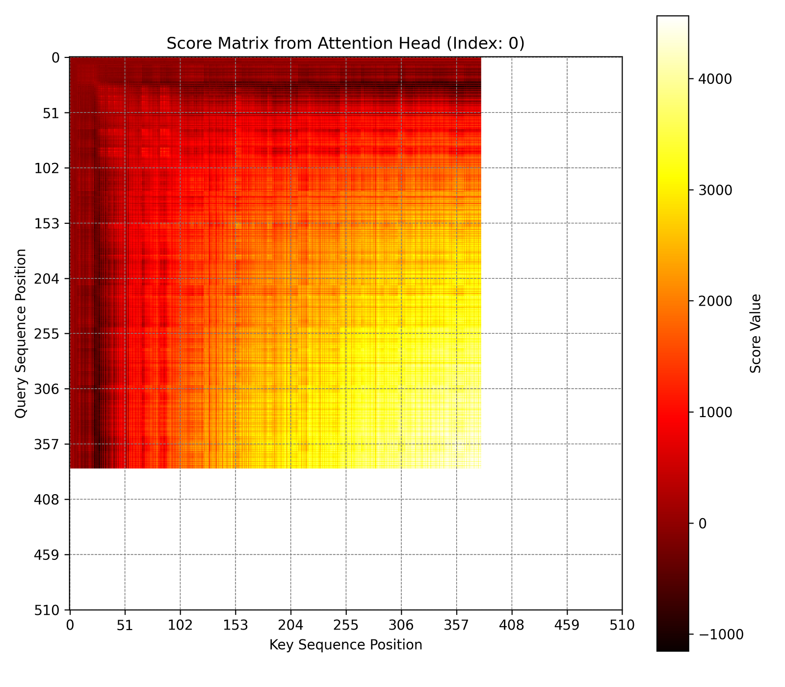
As you can see, the model is not well trained yet and focusses only on only nearby tokens while ignoring far away ones (in red). This makes it difficult to verify the claim. Having said that, it is easier to visualize how, in a fully trained model, such matrix will be dominated by few large values and can be decomposed into a product of 2 smaller matrices. For intuition, imagine you are predicting the next word in a recipe and half the words from the preceding text are dropped. Will you still be able to predict the next word?
Linformer scales linearly in context length as the new scores matrix’s dimension is independent of the context_length. Therefore, its practical benefits in terms of reduced compute and memory are seen for long context lengths (one of the most important features competing LLMs tout).
Implementing Linformer is quite simple. The following code shows the modifications to the existing multi-head attention layer. Since we are also using shared key and query weights, all we need is an extra projection layer. An important change to note is the way we create the causal mask. Rest of the code is the same.
import torch
from torch import nn

class LinformerSharedQK(nn.Module):
    def __init__(
        self,
        num_heads: int,
        embedding_dimension: int,
        causal: bool = True,
        max_context_length: int = 512,
    ):
        super().__init__()
        assert embedding_dimension % num_heads == 0
        self.num_heads = num_heads
        self.head_dimension = embedding_dimension // num_heads

        # Linformer's reduced dimension and corresponding projection layer
        self.qk_reduced_dimension = 64
        self.qk_projection = nn.Linear(max_context_length, self.qk_reduced_dimension, bias=False)

        self.wqkv = nn.Linear(embedding_dimension, 2 * embedding_dimension, bias=False)
        self.score_normalisation_factor = 1.0 / self.head_dimension
        self.softmax = nn.Softmax(dim=-1)
        self.causal = causal

    def forward(self, x):
        self._last_scores = None
        [batch_size, context_length, input_dimension] = x.shape
        device = x.device
        with torch.no_grad():
            if self.causal:
                additive_mask = torch.zeros(
                    (context_length, self.qk_reduced_dimension), device=device
                )
                for i in range(context_length):
                    causal_cutoff_k = min(self.qk_reduced_dimension, i * self.qk_reduced_dimension // context_length + 1)
                    additive_mask[i, causal_cutoff_k:] = float("-inf")
            else:
                additive_mask = torch.zeros(
                    (context_length, self.qk_reduced_dimension), device=device
                )

        qkv = self.wqkv(x).view(
            (batch_size, context_length, self.num_heads, -1)
        )
        qkv = qkv.permute(
            (0, 2, 1, 3)
        )
        query_per_head = qkv[:, :, :, : self.head_dimension]
        key_per_head = query_per_head
        value_per_head = qkv[:, :, :, self.head_dimension :]

        key_for_proj = key_per_head.reshape(
            batch_size * self.num_heads, context_length, self.head_dimension
        )
        key_transposed_for_linear = key_for_proj.transpose(1, 2)

        projected_key_linear_result = self.qk_projection(key_transposed_for_linear)
        projected_key = projected_key_linear_result.transpose(1, 2)

        value_for_proj = value_per_head.reshape(
            batch_size * self.num_heads, context_length, self.head_dimension
        )
        value_transposed_for_linear = value_for_proj.transpose(1, 2)
        projected_value_linear_result = self.qk_projection(value_transposed_for_linear)
        projected_value = projected_value_linear_result.transpose(1, 2)

        query = query_per_head.reshape(batch_size * self.num_heads, context_length, self.head_dimension)
        key = projected_key
        value = projected_value

        key_transpose = torch.transpose(
            key, 1, 2
        )
        scores = torch.bmm(
            query, key_transpose
        )
        masked_scores = scores + additive_mask
        normalised_scores = (
            masked_scores * self.score_normalisation_factor
        )
        attention_probabilities = self.softmax(
            normalised_scores
        )
        self_attention = torch.bmm(attention_probabilities, value)

        return (
            self_attention.view((batch_size, self.num_heads, context_length, -1))
            .permute((0, 2, 1, 3))
            .reshape((batch_size, context_length, -1))
        )
Mixture of Experts
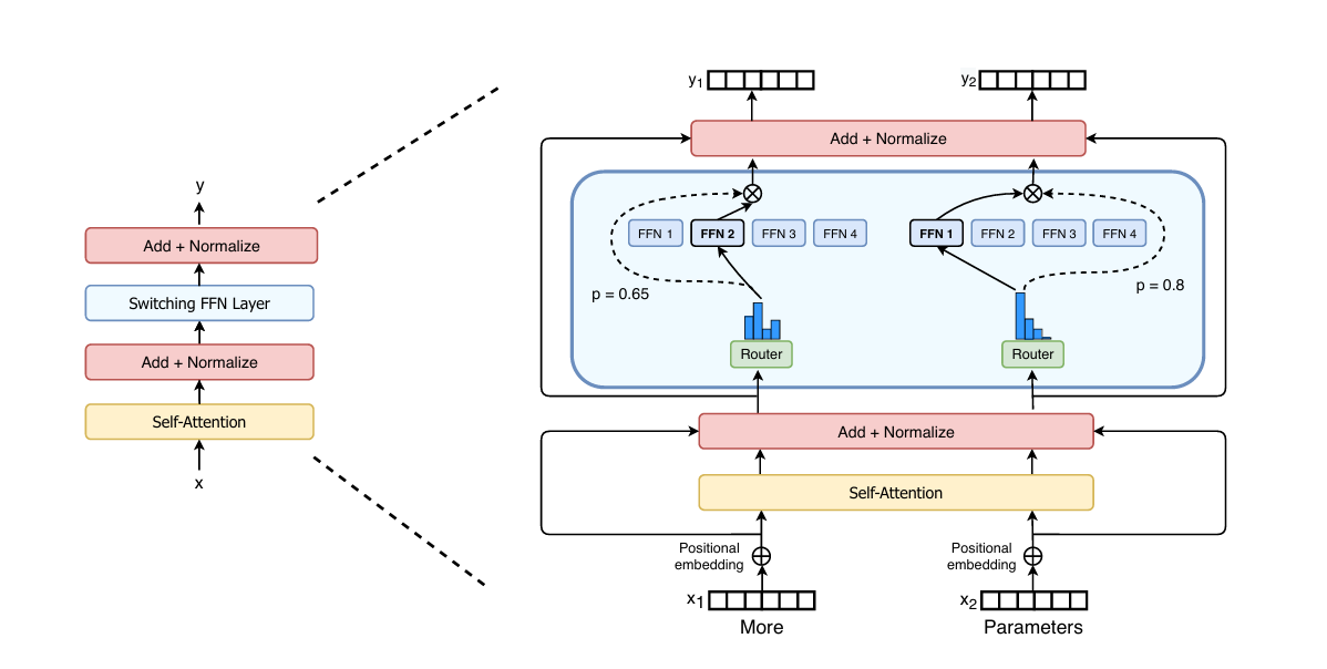
Increasing model capacity is one of the guaranteed ways to improve its performance. Mixture of Experts is a way to increase model capacity without scaling the computation or memory required in the same proportion. Here is a diagram taken from the Switch Transformer paper that shows how MoE can be used to train massive models at a fixed added computation cost.
The idea is quite simple. Instead of having a single MLP block in a transformer block (after attention), we use multiple MLP blocks. Only a few (or even just 1) of them is chosen during the forward pass. Each of those MLP are called the experts and which expert is chosen is decided based on the current token embedding by a simple gating layer (a linear layer followed by a softmax). Experts are chosen independently for each position in the sequence.
Here is a naive implementation of MoE layer that will replace the MLP (linear->GELU->linear) inside each transformer block.
import torch
from torch import nn

class MoE(nn.Module):
    def __init__(self, num_experts: int, embedding_dimension: int):
        super().__init__()
        self.num_experts = num_experts
        self.embedding_dim = embedding_dimension

        # Gating network to select best experts
        self.gate = nn.Linear(embedding_dimension, num_experts)

        # Each expert is the same MLP as vanilla transformer block
        self.experts = nn.ModuleList([
            nn.Sequential(
                nn.Linear(embedding_dimension, 4 * embedding_dimension),
                nn.GELU(),
                nn.Linear(4 * embedding_dimension, embedding_dimension)
            ) for _ in range(num_experts)
        ])

    def forward(self, x: torch.Tensor):
        """
        x: [batch_size, seq_len, embedding_dim]
        Returns: same shape
        """
        batch_size, context_length, embedding_dimension = x.shape # [batch_size, context_length, embedding_dimension]
        x_flat = x.view(-1, embedding_dimension)  # [batch_size * context_length, embedding_dimension]

        # Choose the top 1 expert for each token embedding idependently
        gate_scores = self.gate(x_flat)  # [batch_size * context_length, num_experts]
        top1_expert = torch.argmax(gate_scores, dim=-1)  # [batch_size * context_length]

        # Forward token embeddings to chosen experts
        expert_outputs = torch.zeros_like(x_flat) # [batch_size * context_length, embedding_dimension]
        for i in range(self.num_experts):
            # Get the token indices in x_flat that have chosen the current expert
            expert_mask = (top1_expert == i) # [batch_size * context_length]
            if expert_mask.any(): # Some experts might get 0 token embeddings across all sequences and batches
                selected_input = x_flat[expert_mask]  # token embeddings routed to current expert [Variable, embedding_dimension]
                selected_output = self.experts[i](selected_input) # [Variable, embedding_dimension]
                expert_outputs[expert_mask] = selected_output # [batch_size * context_length, embedding_dimension]

        return expert_outputs.view(batch_size, context_length, embedding_dimension) # [batch_size, context_length, embedding_dimension]
Now in the TransformerBlock constructor, just replace
self.linear = nn.Linear(embedding_dimension, 4 * embedding_dimension)
self.act = nn.GELU()
self.projection = nn.Linear(4 * embedding_dimension, embedding_dimension)
with
self.moe = MoE(num_experts=4, embedding_dimension=embedding_dimension)
and in the forward method, replace
z = self.linear(z) # [batch_size, context_length, embedding_dimension * 4]
z = self.act(z) # [batch_size, context_length, embedding_dimension * 4]
z = self.projection(z) # [batch_size, context_length, embedding_dimension]
with
z = self.moe(z) # [batch_size, context_length, embedding_dimension]
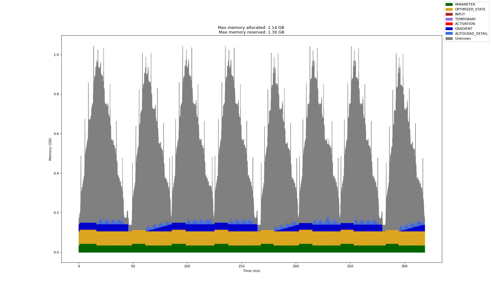
The original model had 3.2 million parameters while the MoE model with four experts has 9.6 million parameters! This is because parameters in dense MLP layers of transformer block are a big fraction of total parameters. Therefore, adding sparsely activated MLP layers scaled the model parameters significantly. The following chart shows the memory profile for training 8 micro batches. Note that even though we had four dense MLPs (an almost 3x increase in number of parameters) in every transformer block, the memory consumed during training was not affected!
The compute time has increased but this can be addressed with a more efficient implementation. A lot of research has gone into figuring out the optimal way to leverage MoE for massive models in a distributed setup.
Going Beyond Model Architecture Optimizations
Even after all such optimizations, MultiheadAttention implementation from PyTorch is still going to outperform our implementations. Below is the trace of the first transformer block using for a micro batch. It shows that the MultiheadAttention_0 module took just 0.421ms (compared to 0.578ms for our implementation of EfficientMultiHeadMaskedSelfAttentionabove). During inference and on certain GPUs and for longer context lengths/embedding dimensions, this gain can be even larger.
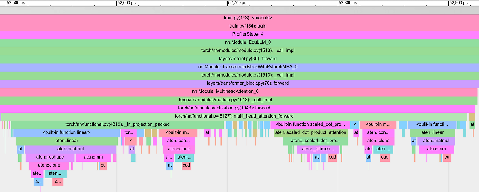
This is because, behind the scenes, it calls scaled_dot_product_attention. This function in PyTorch is logically equivalent to our implementation of multi head attention but is implemented using a combination of mathematical and hardware optimizations.
For instance, scaled_dot_product_attention has three different implementations and the appropriate one is chosen based on the hardware and environment.
- The first is Memory Efficient Attention. This is an exact implementation of attention (unlike Linformer which approximates it) but uses a mathematical trick to reduce memory consumption to linear complexity (the time complexity stays quadratic).
- Another implementation, and the most popularly used, is FlashAttention. This is a GPU memory and programming model aware implementation that also achieves linear memory complexity along with runtime speed ups.
- Third is a C++ implementation of attention that is invoked from Python code.
In essence, while our EfficientMultiHeadMaskedSelfAttention implementation is optimized for parallelism by batching the heads, PyTorch's scaled_dot_product_attention takes it a step further by optimizing the underlying sequence of arithmetic operations themselves. This makes it highly efficient, especially for larger models and long context lengths where memory bandwidth and computation efficiency becomes paramount.
We shall learn more about these techniques in another blog post. Till then, torch.nn.MultiheadAttention should be the ideal implementation you would need in practice.