
Optimizing the Training Loop
In previous posts, we built a data collection pipeline and trained a byte pair encoder tailored to our data for our custom LLM training. Before, we define the LLM architecture, let’s dive into some optimization techniques that will help us save (a lot of) time and money.
The diagram below is a chart from the paper Scaling Laws for Neural Language Models by OpenAI. The paper examines the test performance of a trained Language Model in relation to the model’s size, data volume, training duration, and model shape.
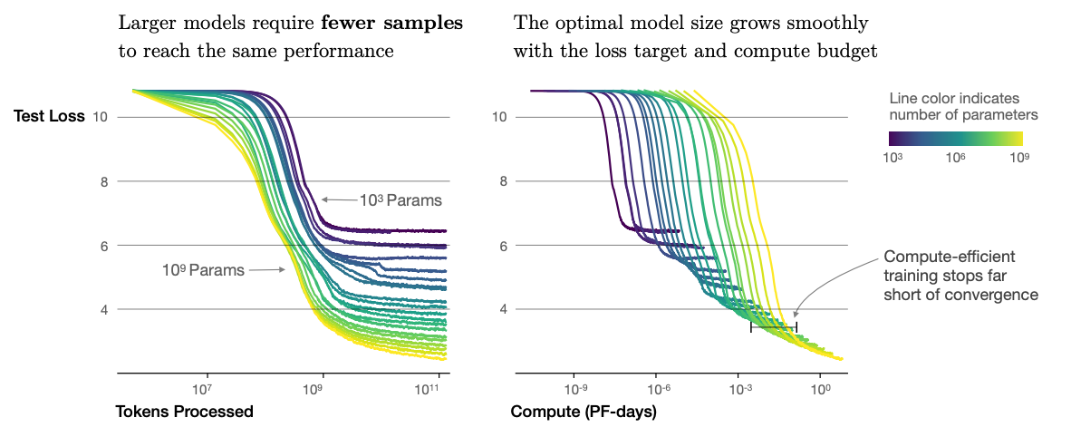
The chart on the right has the horizontal axis in PF-days (1 PF-day is equal to $8.64 \times 10^{19}$ FLOPs (FLoating point OPerations)). The vertical axis shows the test loss which is categorical cross entropy between predictions and ground truth from the test dataset.
The chart shows that models with fewer parameters converge at a higher test loss, irrespective of how long you train them. Based on the chart, it is preferable (in terms of test loss) to use a larger model and stop early (before convergence) rather than training a smaller model to convergence. To reach a test loss of 4 or below, we need a minimum of $10^{-3}$ PF-days with a model having at least ~$10^{8}$ parameters (100 million). For reference, GPT-2 is a 1.5 billion parameter model. When trained to convergence, it achieves a test loss of ~1.5.
To reach the level of GPT-2 (test loss of 1.5 or below), the chart says we need at least a billion ($10^{9}$) parameter model trained for $10^{0} = 1$ PF-days ($8.64 \times 10^{19}$ FLOPS). A single A100 GPU can run at $0.195 \times 10^{14}$ FLOPS if operating in 32 bit floating point precision. Which means, we need to train a billion parameter model (in 32 bit precision) for at least 4,430,769 seconds (approximately 7 weeks). And this assumes that we utilize the GPU at its peak performance.
Even when you're not training language models, determining the right hyperparameters for a deep learning model is an iterative process involving pseudo-random exploration based on intuition. Errors in code often fail silently. Therefore, it's crucial to run experiments quickly to save both time and money.
All of this demonstrates the importance of optimizing model training in terms of time and compute. In other words, we must optimize our code to achieve the following:
1. Minimize the GPU time (number of GPUs multiplied by the usage time of each GPU) needed to train the model by reducing the memory used by the model and optimizer during training.
2. Ensure the GPUs operate near their peak compute capacity throughout training.
In this post, we shall explore some model architecture independent optimizations that will enable us to train almost 10 times faster with 10 times lower memory footprint. The techniques demonstrated in this post are applicable to any deep learning model/task - not just LLMs. We will look at the model as a black box and optimize just the training loop.
To ground the discussion, we shall use a small, GPT style, decoder only transformer model with approximately three million parameters and a reference task of next token prediction with teacher forcing. Also, we will use PyTorch throughout the discussion. This will allow us to use profiling tools to accurately measure the performance improvements corresponding to every change. The implementation of the model will be detailed in the next post along with model architecture specific optimizations.
Let's start by implementing a typical training loop.
# Copy model to correct device
model = model.to(device)
for epoch in range(num_epochs):
  for batch, (inputs, targets) in enumerate(train_dataloader):
    # Copy tensors to correct device
    inputs, targets = inputs.to(device), targets.to(device)
    # Forward pass
    preds = model(inputs, train=True)
    # Compute loss
    loss = cross_entropy(
        preds.view(-1, preds.size(-1)),
        targets.view(-1),
        ignore_index=PADDING_TOKEN_ID,
        reduction="mean",
    )
    # Backward pass to compute and accumulate gradients
    loss.backward()
    print(f"Loss: {loss.item()}")
    # Descend the gradient one step
    optimizer.step()
    # Set the stored gradients to 0
    optimizer.zero_grad()
Here targets and inputs are a batch of sequences of token ids having the shape [batch_size, context_length, 1]. For next token prediction with teacher forcing, the target sequences are just input sequences shifted by one token. In case the sequence length is less than context_length, the rest of the positions are filled with PADDING_TOKEN_ID. The predictions preds are logits of shape [batch_size, context_length, vocabulary_size] . The cross entropy is computed independently for each pair of predicted token probabilities and target token id and then averaged across the batch and sequence dimensions. Therefore, the predictions can be flattened into shape [batch_size * context_length, vocabulary_size] and the targets can be flattened into shape [batch_size * context_length, 1] . Refer to the documentation of torch.nn.functional.cross_entropy for further details on the expected inputs.
As we shall see in the next post, the model will operate on all tokens and make predictions for all positions (even the positions filled with PADDING_TOKEN_ID ). Instead, the cross-entropy loss function will ignore the positions where original sequence had the PADDING_TOKEN_ID. Therefore, there’s no need to mask the inputs or targets during the forward pass, and yet the padded positions do not contribute to the final loss.
Note that in this case, the device has to store at least -
| Tensors | Number of values to store is proportional to |
|---|---|
| inputs | batch_size * context_length * 1 |
| targets | batch_size * context_length * 1 |
| preds | batch_size * context_length * vocabulary_size |
| activations | depends on model architecture and its computation graph |
| gradients | num_params |
| model parameters | num_params |
| Optimiser states like momentum | num_params * num_states_per_parameter |
Note that, for a 117 million parameter GPT-2-small model, the gradients, model parameters and optimiser states will consume just $4 \times 117 \times 10^6 \times 3 = 1.4\text{ Gb}$ of memory (assuming one state number per parameter for optimiser and all numbers being stored in 32 bit floating point precision). The data consumes a negligible amount in comparison.
Yet, while training with a single GPU of 32 Gb memory capacity, the program will throw out of memory exceptions. This is because storing the activations can require an order of magnitude more memory than the rest of the tensors combined.
The number of activation values stored during forward pass is difficult to compute. In automatic differentiation, during forward pass, every operation needs to store some data it would need for computing gradients during backward pass using chain rule. For example, in case of matrix multiplication of an input matrix with a weight matrix, automatic differentiation needs to store the input matrix to compute gradient of output values with respect to the weight matrix values during backward pass. In case of activation like softmax, we need to store the output of softmax to compute the gradient of output values with respect to the input matrix values. The number of activation values stored depends on the operations in computation graph and the input/output shapes of each.
In case of transformers, the paper Reducing Activation Recomputation in Large Transformer Models by Nvidia gives a good formula for estimating the activation memory of a transformer block. According to that paper, a single standard transformer block using 32-bit floating point numbers requires
$$2sbh\left(34 + \frac{5as}{h}\right)$$
where $s$ is the context length, $h$ is the embedding dimension, $b$ is the batch size and $a$ is the number of attention heads.
The GPT-2-small configuration uses 12 transformer blocks with $s = 1024$, $h = 768$, $b = 32$, and $a = 12$. Which means the peak memory usage should be close to 69 Gb! The initial learnt positional embeddings and word embeddings (shared with final projection layer) would use a few additional Mbs.
By the end of this post, we should be able to train a GPT-2-small sized model (or even larger) on a single GPU almost 10 times faster than a naive PyTorch training loop implemented above.
In order to iterate and profile faster, we shall use a smaller reference architecture with just four transformer blocks having $s = 512$, $h = 256$, $b = 32$, and $a = 4$. With this model configuration, our peak memory usage for the naive version should be close to 2.5 Gb.
Gradient Accumulation
Lets start with basic memory optimizations. First, optimizer.zero_grad() allows a parameter set_to_none. When set_to_none is True, the gradient is set to None instead of a tensor of 0s thus saving a modest amount of memory. But it still does not change the peak memory usage. You only need to exceed memory once for the script to crash.
Note that the activation memory depends on batch size. To reduce peak memory usage, we can use a simple technique called gradient accumulation. Note that for a batch size of $N$ samples $x_1, x_2, ..., x_N$,
$$
\frac{\text{d}(loss)}{\text{d}W} = \frac{1}{N}\left(\frac{\text{d}(loss(x_1))}{\text{d}W} + \frac{\text{d}(loss(x_2))}{\text{d}W} + ... + \frac{\text{d}(loss(x_N))}{\text{d}W}\right)
$$
Therefore, instead of feeding all $N$ samples of a batch during the forward pass, we could forward one sample at a time and accumulate the gradients for that sample. The accumulated gradient over all samples of a batch can then be divided by $N$ to give the final gradient. This gradient value should be exactly equal to the gradient computed by feeding the entire batch at once (barring numerical precision issues). This way, we get to use a large batch size ($N$) for gradient descent and yet the peak activation memory drops by a factor of $N$.
This technique will result in increased computation time as samples are now processed in a loop. Therefore, to strike a balance, we can divide the batch into micro batches of just enough samples to fit into the GPU memory.
Lets re-write the training loop with gradient accumulation.
gradient_accumulation_steps = 4
# Copy model to correct device
model = model.to(device)
for epoch in range(num_epochs):
  for batch, (inputs, targets) in enumerate(train_dataloader):
    # Divide a batch into micro batches
    for micro_batch_step in range(gradient_accumulation_steps):
      micro_batch_size = inputs.shape[0] // gradient_accumulation_steps
      start, end = (
          micro_batch_step * micro_batch_size,
          (micro_batch_step + 1) * micro_batch_size,
      )
      # Copy micro batch tensors to correct device
      micro_batch_inputs = inputs[start:end, :].to(device)
      micro_batch_targets = targets[start:end, :, :].to(device)
      # Forward pass
      preds = model(micro_batch_inputs, train=True)
      # Compute loss
      loss = cross_entropy(
          preds.view(-1, preds.size(-1)),
          micro_batch_targets.view(-1),
          ignore_index=PADDING_TOKEN_ID,
          reduction="mean",
      )
      # Scale loss
      loss = loss / gradient_accumulation_steps
      # Backward pass to compute and accumulate gradients
      loss.backward()
      print(f"Loss: {loss.item()}")
    # Descend the gradient one step
    optimizer.step()
    # Set the stored gradients to None to free memory
    optimizer.zero_grad(set_to_none=True)
In this case, all memory requirements proportional to batch_size decreases by a factor of gradient_accumulation_steps. This includes activation memory. This allows us to scale the model, use longer context or increase the batch size.
Profiling
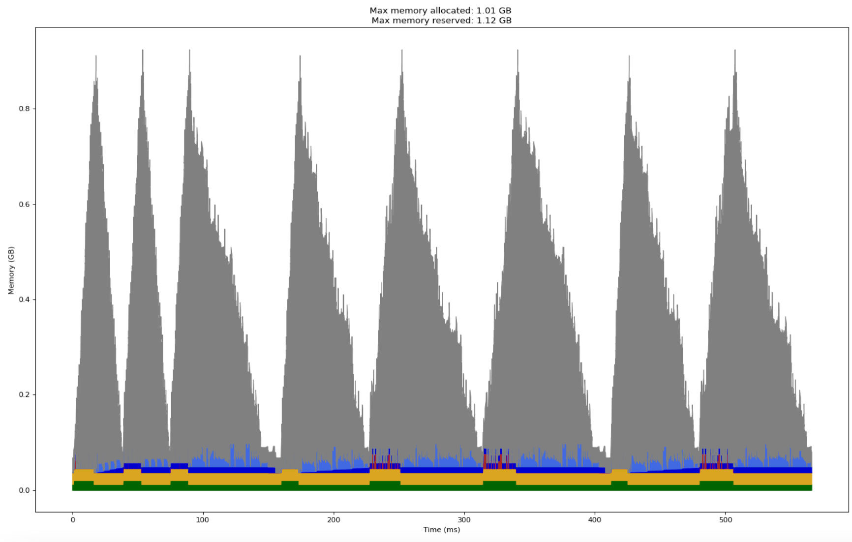
The following chart shows the memory profile of the training loop on two batches of data (2*gradient_accumulation_steps steps)
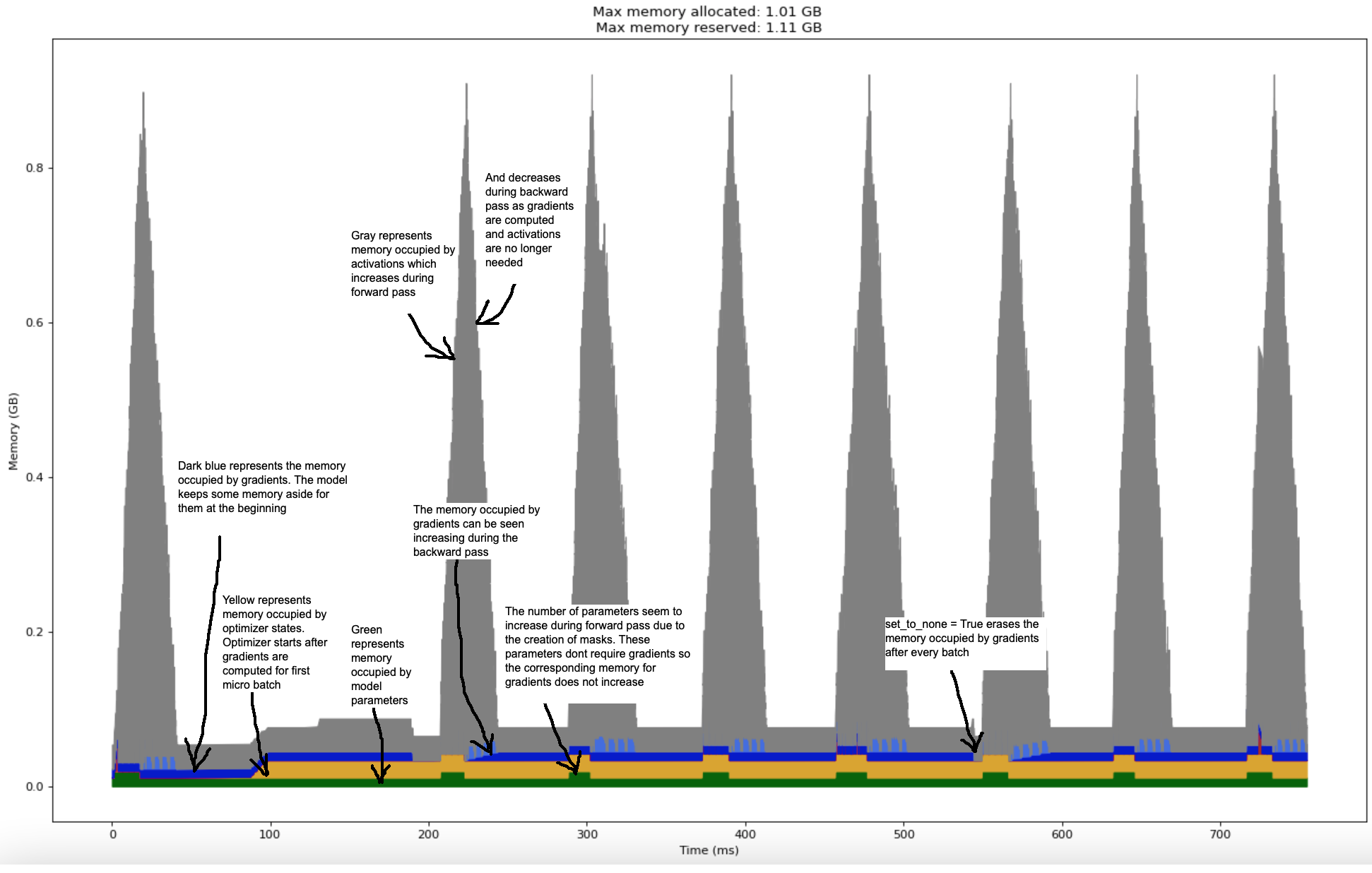
We can see that the peak memory usage for the model is close to 1.11 Gb.
The model has 3,024,384 parameters and we operate in 32 bit (4 byte) floating point numbers. Which means the model parameters (shown as green in the chart) should occupy about 3,000,000 * 4 bytes which is approximately 12 Mb. The gradients (shown as royal blue in the chart) should occupy similar memory since gradients stores one number per parameter too (or multiple in case of optimizers like Adam). The calculated numbers correspond well with the chart above.
The number of activation values stored during forward pass, according to the previous formula, should be close to 620 Mb. The initial learnt positional embeddings and word embeddings (shared with final projection layer) would use a few aditional Mbs. The number seems to be in the same ballpark as the chart (the gray region which shows approximately 850 Mb of activation and other intermediate tensor peak memory).
Mixed Precision Training
Another straightforward optimisation is to use lower presicion to store some numbers. By using 16-bit floating point numbers instead of 32-bit, we can reduce the memory usage as well as increase the speed. But some operations (like taking a step in the opposite direction of gradient) are affected more by the loss in precision compared to other operations (like matrix multiplication). Therefore, to prevent a loss in quality, we need to train the model in mixed precision by using lower presion numbers whenever acceptable. The torch.amp module provides convinient APIs to leverage mixed-precision training without any change to the model definition.
Lets re-write the training loop with gradient accumulation and mixed precision training.
gradient_accumulation_steps = 4
# Copy model to correct device
model = model.to(device)
for epoch in range(num_epochs):
  for batch, (inputs, targets) in enumerate(train_dataloader):
    # Divide a batch into micro batches
    for micro_batch_step in range(gradient_accumulation_steps):
      micro_batch_size = inputs.shape[0] // gradient_accumulation_steps
      start, end = (
          micro_batch_step * micro_batch_size,
          (micro_batch_step + 1) * micro_batch_size,
      )
      # Copy micro batch tensors to correct device
      micro_batch_inputs = inputs[start:end, :].to(device)
      micro_batch_targets = targets[start:end, :, :].to(device)
      with torch.autocast(device_type=device):
        # Forward pass
        preds = model(micro_batch_inputs, train=True)
        # Compute loss
        loss = cross_entropy(
            preds.view(-1, preds.size(-1)),
            micro_batch_targets.view(-1),
            ignore_index=PADDING_TOKEN_ID,
            reduction="mean",
        )
        # Scale loss
        loss = loss / gradient_accumulation_steps
        loss = scaler.scale(loss)
        # Backward pass to compute and accumulate gradients
        loss.backward()
        print(f"Loss: {loss.item()}")
    # Descend the gradient one step
    scaler.step(optimizer)
    scaler.update()
    # Set the stored gradients to None to free memory
    optimizer.zero_grad(set_to_none=True)
Since mixed precision training affects output quality, we can’t just compare its memory/compute profile. We need to compare its test performance too. Therefore, we will continue futher optimisations for full 32 bit precision training.
Recent Nvidia GPUs have introduced new floating point representations that offer a balance between range and precision that is more suitable for deep learning. For example, TF32 is a special datatype supported on Ampere (and later) architecture GPUs to speed up multiply-accumulate operations commonly used in matrix multiplications. The tensor cores in these GPUs can round FP32 inputs to TF32, perform fast multiplication and accumulate the result back in FP32. If your GPU has Ampere or later architecture (nvidia-smi command line utility can help you identify your Nvidia GPU’s architecture), you could add the following two lines at the beginning of your program to leverage them.
torch.backends.cuda.matmul.allow_tf32 = True
torch.backends.cudnn.allow_tf32 = True
Gradient Checkpointing
As seen previously, bulk of the memory is occupied by tensors stored during forward pass that are required to compute gradients during backward pass. If we avoid storing these and instead re-compute them during backward pass, we could probably run a 10x (or even larger) sized model on a single GPU! But note that, for every operation, we would have to do a partial forward pass from the inputs till that operation during backward pass which will increase the compute time of the backward pass quadratically.
An intelligent gradient checkpointing scheme will save a subset of tensors as checkpoints through the computation graph so that the partial forward passes do not have to start from the inputs. This method is called gradient checkpointing. The general problem to solve for any gradient checkpointing scheme is as follows -
Given
- An arbitrary computation graph,
- Compute time associated with every operation node in the graph,
- The memory required to store the intermediate tensor for that node,
- And a given memory limit,
Find the tensors that should be stored during forward pass (should fit within the memory limit) that will minimize the compute time during the backward pass.
The problem is quite challenging to solve efficiently. Simplified versions are usually solved using dynamic programming.
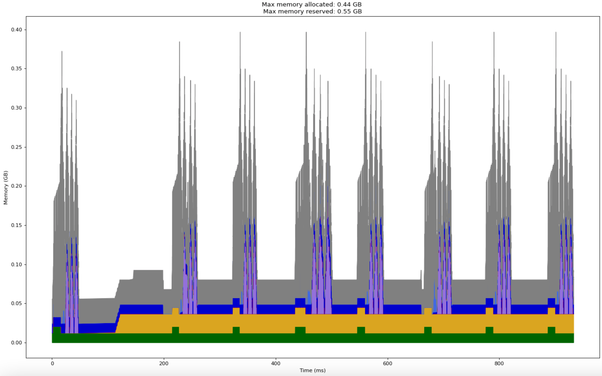
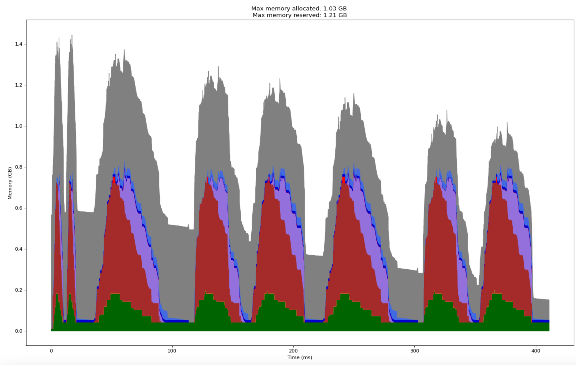
Following chart shows the memory profile of the same model and hyper parameters with gradient checkpointing. In this case, the input to each transformer block is stored as a checkpoint. Therefore, in every micro batch, we see four rising and dropping spikes. The initial rise (up to approximately 0.2 Gb) before the first spike corresponds to the models forward pass. Post the forward pass, we see four spikes of approximately 150 Mb corresponding to the extra forward passes made for each transformer block during backward pass gradient computation. The 150 Mb number matches well with the previous formula for activation memory required for a single transformer block.
Note that we reduced the model’s peak memory reserved by half while increasing the compute time by merely 25% (two batches in this case took 1000 ms compared to 800 ms without gradient checkpointing). With an appropriately designed checkpointing strategy, you could fit 10x larger model for less than 50% processing time increase.
PyTorch does provide an API to use gradient checkpointing in your model (which was used to produce this chart). But using it is not as straightforward unless you have a simple sequential model. For example, if your model uses a dropout layer, a checkpoint needs to be set immediately before and after the dropout layer since dropout will mask different random inputs on every forward pass. Similarly, with batch normalization layer, each forward pass will update the batch normalization mean and standard deviation parameters. Therefore, performing extra forward passes for computing gradients can lead to hard to debug quality degradations.
Since the model used in this case involves dropout and layer normalization, the strategy used in this chart (to checkpoint each transformer block) will lead to incorrect training. The checkpointing strategy shown here is just meant to demonstrate the effectiveness of its compute-memory trade off. Appropriate strategy must be manually designed based on the model architecture.
Optimizing I/O
If you observe the profile charts till now, you can see that there is a long gap of low memory consumption between the end of backward pass of one micro batch and the start of forward pass of the next micro batch. What exactly is being computed in that gap?
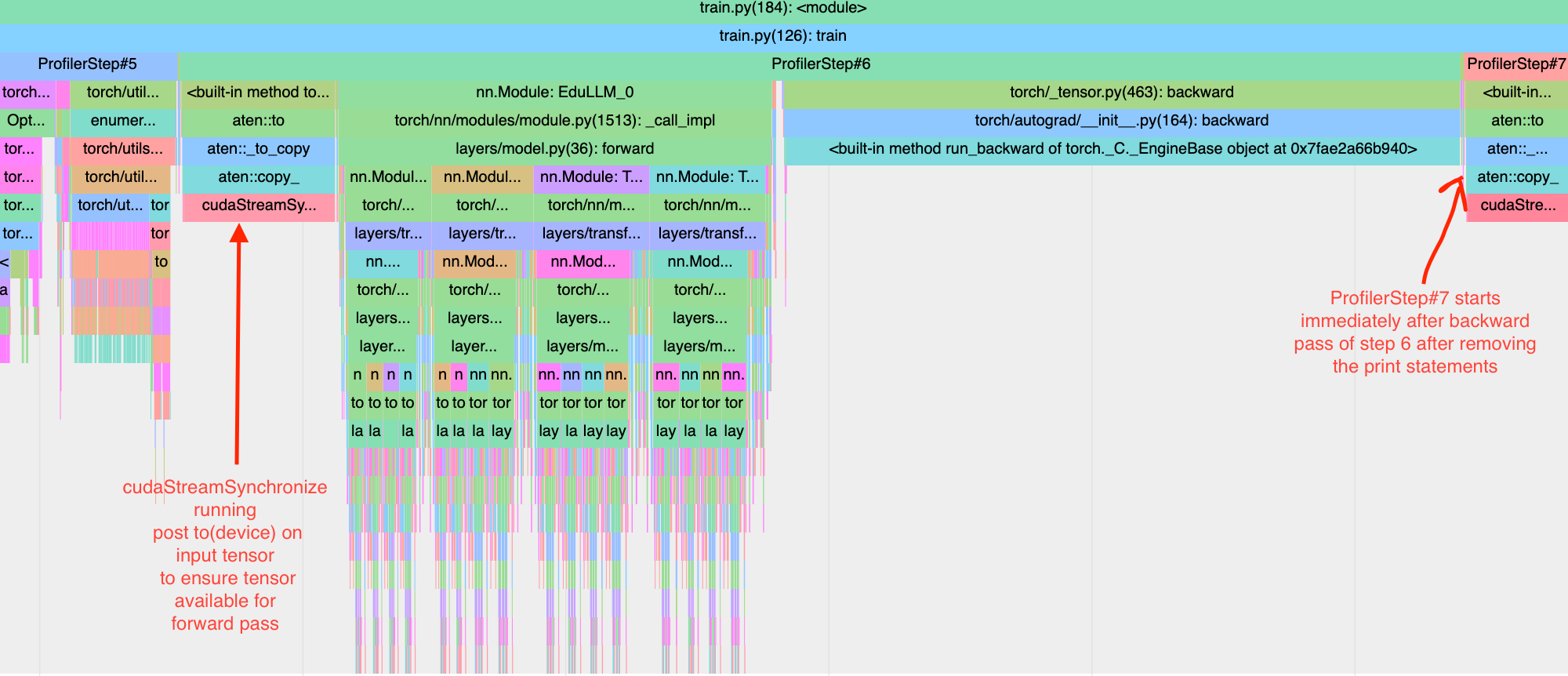
To understand that, we can look at the chrome trace of one micro batch iteration marked by ProfilerStep#6.
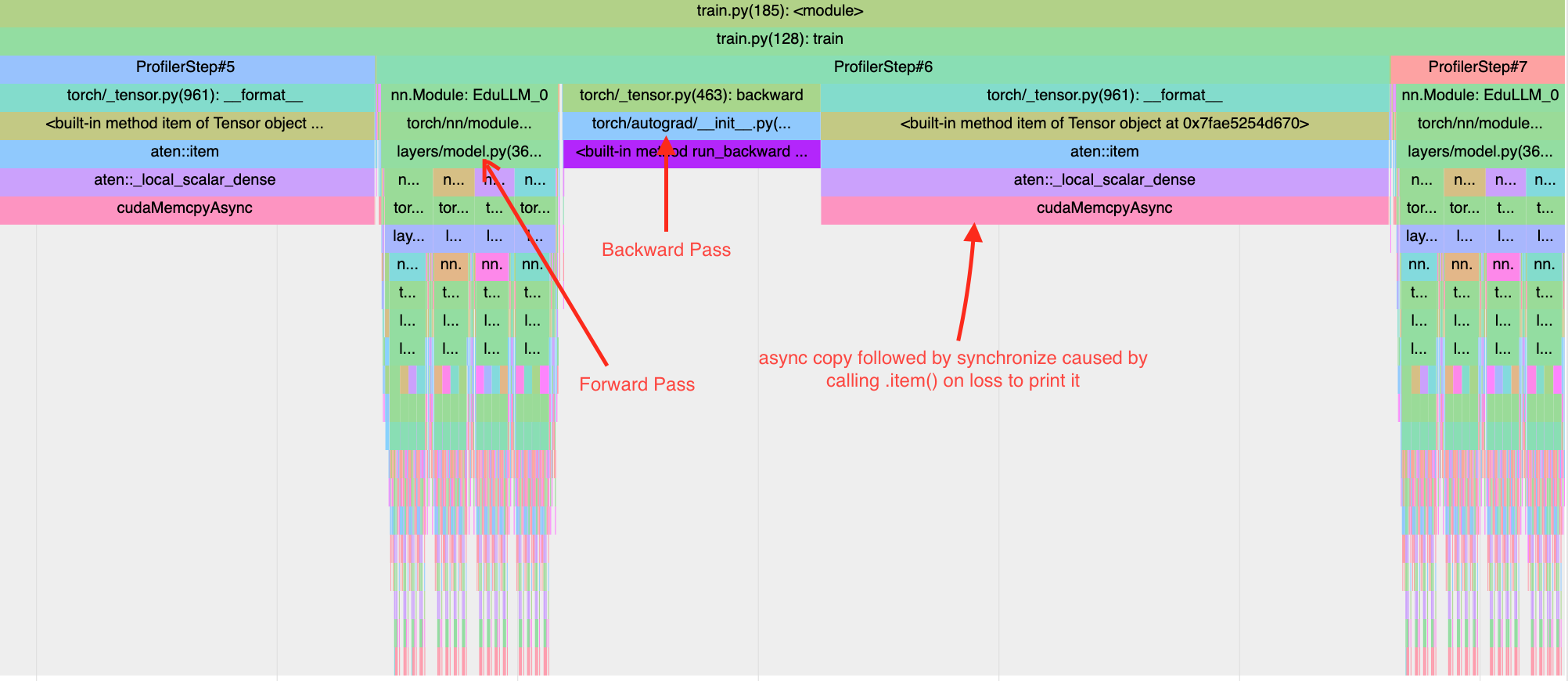
From the trace, we can see that a significant time is spent copying a tensor (loss value tensor in this case) back to the CPU. The statement print(f”Loss: {loss.item()}”) causes copying of loss tensor from GPU to CPU and the program waits till the copy is finished. So the first thing we should target is removing statements that explicitly cause copying of tensors between devices - like print statements and writing scalars to tensorboard within the micro batch loop.
But note that in the same chart, copying micro batches from CPU to GPU does not seem to take much time. In above chart, it happens in the very narrow gap between where ProfilerStep#5 ends and where forward pass of ProfilerStep#6 starts. The situation is a bit more nuanced than what the chart shows. Here is the same profiler step after removing the print statements. We can now see that while the gap post backward pass of ProfilerStep#6 has disappeared, a modest gap for tensor.to(device) (specifically cudaStreamSynchronise) has appeared before the forward pass of of ProfilerStep#6 (the forward pass needs the input tensor before executing). To understand why it did not show up in the previous chart needs a more detailed understanding of CUDA streams and tensor copy within CUDA. This blog article by Nvidia explains it well.
As a rule of thumb, I/O operations are usually much slower than compute. They are also independent in the sense that a computer can perform those parallelly with instruction executions.
Therefore, instead of sequentially copying data to the device and then performing a forward-backward pass, we could overlap these operations by -
- Copying first batch to the device asynchronously. Set this as the current batch.
- Asynchronously start copying next batch on the device and begin processing current batch without waiting for the next copy operation to finish.
- Loop back to step 2.
The following code shows the modified loop. Note that to use non_blocking=True in to(…) method, the dataloader needs to be created with pin_memory=True
gradient_accumulation_steps = 4
# Copy model to correct device
model = model.to(device)
for epoch in range(num_epochs):
  for batch, (inputs, targets) in enumerate(train_dataloader):
    micro_batch_size = inputs.shape[0] // gradient_accumulation_steps
    # Copy first micro batch
    micro_batch_inputs = inputs[:micro_batch_size, :].to(device, non_blocking=True)
    micro_batch_targets = targets[:micro_batch_size, :, :].to(device, non_blocking=True)
    # Divide a batch into micro batches
    for micro_batch_step in range(1, gradient_accumulation_steps):
      start, end = (
        micro_batch_step * micro_batch_size,
        (micro_batch_step + 1) * micro_batch_size,
      )
      # Asynchronously copy next micro batch tensors to
      # correct device before processing current micro batch
      next_micro_batch_inputs = inputs[start:end, :].to(device, non_blocking=True)
      next_micro_batch_targets = targets[start:end, :, :].to(device, non_blocking=True)

      # Forward pass on current micro batch
      preds = model(micro_batch_inputs, train=True)
      # Compute loss
      loss = cross_entropy(
        preds.view(-1, preds.size(-1)),
        micro_batch_targets.view(-1),
        ignore_index=PADDING_TOKEN_ID,
        reduction="mean",
      )
      # Scale loss
      loss = loss / gradient_accumulation_steps
      # Backward pass to compute and accumulate gradients
      loss.backward()
      # Set current micro batch to next micro batch
      micro_batch_inputs = next_micro_batch_inputs
      micro_batch_targets = next_micro_batch_targets
    # Final micro batch
    preds = model(micro_batch_inputs, train=True)
    loss = cross_entropy(
      preds.view(-1, preds.size(-1)),
      micro_batch_targets.view(-1),
      ignore_index=PADDING_TOKEN_ID,
      reduction="mean",
    )
    loss = loss / gradient_accumulation_steps
    loss.backward()

    # Descend the gradient one step
    optimizer.step()
    # Set the stored gradients to None to free memory
    optimizer.zero_grad(set_to_none=True)
If compute and I/O take similar time, the runtime could be reduced by a significant factor with such a procedure. Here is the performance profile after the above asynchronous copy modifications. The execution time has dropped by more than 25%! Memory consumption does not change.
Although we used an LLM as reference model, the optimizations involved till now were applied to the training loop and made no specific assumptions about the model architecture. All of those techniques could be used with any deep learning model.
Also note that all above optimizations were independent and can be combined to gain significant speed ups and memory efficiency. An optimized training loop for large models training on a single GPU will often combine -
- Gradient accumulation
- Mixed precision training with device specific efficient floating point representations
- Gradient checkpointing
- Asynchronous I/O
Profiling tools should be used to find bugs and the right hyperparameters for such optimizations.
Use a Compiler!
If you thought this was the end of model architecture independent optimizations, then here is a one-line trick that can drop compute time by additional 30% while barely consuming any additional memory. Just add -
model = torch.compile(model)
Two iterations of training loop with this one line change took approximately 400 ms.
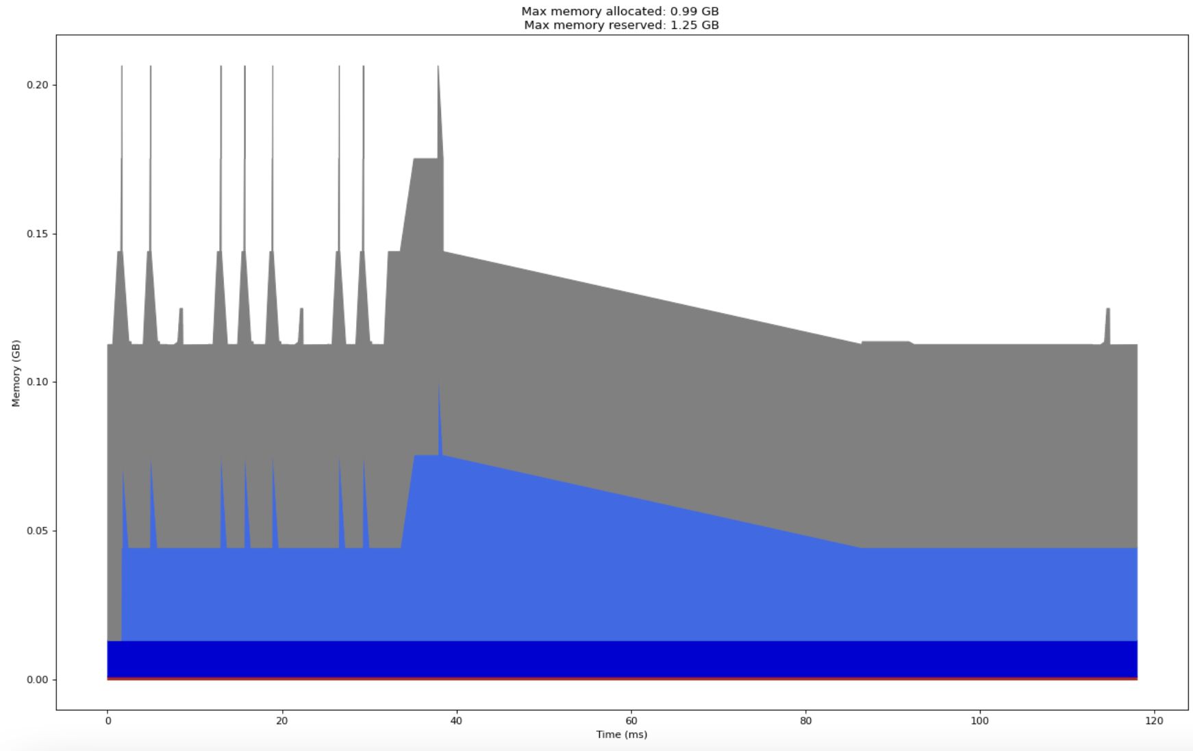
And here is a modification to that one line that will further drop it by almost 75%!
model = torch.compile(model, mode="max-autotune")
At this stage, the profile graph looks really weird and does not offer much information apart from the fact that the training loop on the same two batches took less than 120 ms!
A lot happens behind the scenes with the addition of that single line. We will explore all of that when we delve into compilers in upcoming posts. At that point, we will also explore some domain specific programming languages whose compilers are particularly designed for deep learning style workloads on specialized GPUs. With such DSLs, we can potentially obtain speeds even faster than torch.compile compiled code.
As promised, here is the profile for full 117 million parameter GPT-2-small training with a batch size of 32 and just a subset of optimizations -
- Asynchronous I/O.
- Four gradient accumulation steps.
- And torch.compile with default parameters.
The resulting model takes 7 seconds for two batches and consumes just 10 Gb peak memory!
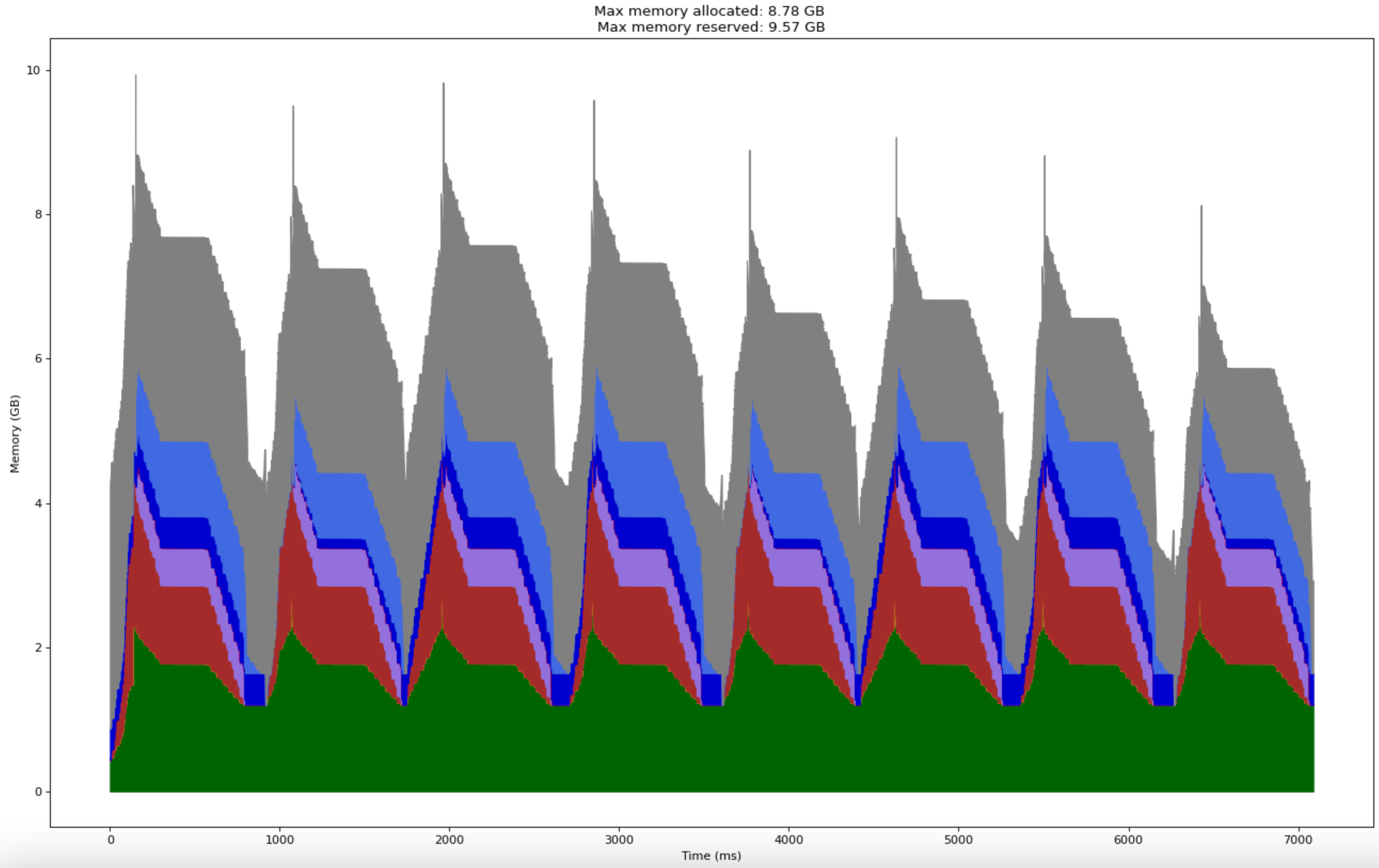
By making small tweaks to our training loop, we were able to train GPT-2-small on a single GPU with loads of memory to spare!
Next Steps
In the upcoming posts, we shall discuss -
- Even more optimizations, but specific to an LLM model architecture.
- Explore PyTorch compilers and some domain specific compiled languages for optimized deep learning on GPUs.
- Explore distributed training with multiple GPUs that will allow us to train multi-billion parameter models.